Download

1 / 9
90 likes | 347 Views
Lecture 6: Aliasing Sections 1.6. Key Points. Two continuous-time sinusoids having different frequencies f and f (Hz) may, when sampled at the same sampling rate f s , produce sample sequences having effectively the same frequency. This phenomenon is known as aliasing, and occurs when

E N D
Key Points • Two continuous-time sinusoids having different frequencies f and f (Hz) may, when sampled at the same sampling rate fs, produce sample sequences having effectively the same frequency. This phenomenon is known as aliasing, and occurs when f ± f= kfs for some integer k. • If a continuous-time signal consisting of additive sinusoidal components is sampled uniformly, reconstruction of that signal from its samples is impossible if aliasing has occurred between any two components at different frequencies. • If the sinusoidal components of a continuous-time signal span the frequency range 0 to fB (Hz), aliasing is avoided if and only if the sampling rate fs exceeds 2fB, a figure known as the Nyquist rate
Review • We saw that a continuous-time sinusoid of frequency f =1/T (Hz) can be sampled at two different rates fs =1/Ts and f=1/Tsto produce sample sequences having the same effectivefrequency. • This happens whenever Ts ± Ts= kT for some integer k.
Aliasing • An analogous phenomenon occurs when two continuous-time sinusoids having different frequencies f and fare sampled at the same rate fs: • depending on the value of fs, the two sample sequences may have the same effective frequency. • When this happens, we say that f and f are aliases (of each other) with respect to the sampling rate fs. • In mathematical terms, we know that ω =2π f/fs and ω=2π f /fs • can be used to represent the same discrete-time sinusoid provided ω = ±ω +2kπ for some integer k. Thus f and f are aliases with respect to fs provided f ± f = kfs
Example • Let f = 150 Hz and fs = 400 samples/sec. Then the aliases of f are given (in Hz) by f = 150 + k(400) and f = −150 + k(400) • If we reduce fs to 280 samples/sec, then the aliases of f are given by f = 150 + k(280) and f = −150 + k(280) • Your task: In each case (fs = 400 and fs = 280), determine all the aliases in the range 0 to 2,000 Hz.
Example • Suppose that x(t) is a sinusoid whose frequency is between 600 and 800 Hz. It is sampled at a rate fs = 400 samples/sec to produce x[n]=4.2 cos(0.75πn − 0.3) • This information suffices to determine x(t), i.e., reconstruct the signal from its samples. First, we note that 2πf/fs=0.75π ⇒ f = (0.375)(400) = 150 Hz which is outside the given frequency range. From the previous example, the only alias of f in the range [600, 800] Hz is f = 650 Hz. This is the correct frequency for x(t), and x(t)=4.2 cos(1300πt +0.3) • Question: Why was the initial phase inverted (between x(t) and x[n])?
Analog-to-Digital Conversion • Analog-to-digital conversion involves sampling a signal x(t) at a rate fs and storing the samples in digital form (i.e., using finite precision). Digital-to-analog conversion is the reverse process of reconstructing x(t) from its samples. If x(t) is a sum of many sinusoidal components, then faithful reconstruction is impossible if aliasing has taken place, i.e., if two or more components of x(t) have frequencies which are aliases of each other with respect of fs. • Your task: Convince yourself that this is so by revisiting the previous example. If the same sample sequence x[n] had represented the sum of two sinusoids in continuous time, at frequencies 150 and 650 Hz, could you have written an equation for x(t) using the given formula for x[n] only?
Avoiding Aliasing • When sampling a signal x(t) containing many different frequencies in the range [0,fB] Hz (B here stands for bandwidth), aliasing can be avoided if the sampling rate is greater than 2fB. One way of showing this is by plotting all aliases of frequencies in the given range [0,fB], using the equations derived earlier: f = f + kfs (top axis) and f = −f + kfs (bottom axis) • Each value of k corresponds to a translate of [0,fB] on the frequency axis. Aliasing is avoided when no two bands overlap (except at multiples of fs). This is ensured if fs > 2fB. • Your task: Explain why aliasing occurs when fs =2fB − δ, where δ is positive amount less than, say, fB. Find two frequencies in the interval [0,fB] that are aliases of each other with respect to fs.