Download

1 / 41
430 likes | 699 Views
FREstimate Software Quick Start Guide. Ann Marie Neufelder SoftRel, LLC www.softrel.com amneufelder@softrel.com. Helpful information. Press F1 key at any time to see relevant help Mouse over fields to see tooltips Electronic copies of the user’s manuals can be found at

E N D
FREstimate Software Quick Start Guide Ann Marie Neufelder SoftRel, LLC www.softrel.com amneufelder@softrel.com
Helpful information • Press F1 key at any time to see relevant help • Mouse over fields to see tooltips • Electronic copies of the user’s manuals can be found at • http://www.softrel.com/support.htm
Tips for Installing FREstimate • Install on a recent Windows Operating System • If you are installing onto Vista • a. Save the installation file to your hard drive instead of installing from the internet • b. Right click on the download file and select "Run as adminstrator“ • c. After installation you will need to download this application to support the Frestimate help files • http://www.microsoft.com/downloads/details.aspx?FamilyID=6ebcfad9-d3f5-4365-8070-334cd175d4bb&DisplayLang=en • Shut down all other programs prior to installing • Log in to Windows as a user with system admin privileges as the install process requires write access to the windows/system32 folder • Do not install on a network drive or any drive that you do not have write privileges for • It is recommended that you install onto a “C:” drive • If you notice any error messages during installation, write them down and continue with the install. You may notice error messages if you are installing over a previous version of Frestimate. • After the software is successfully installed, you can launch it from Windows Start->All programs or by launching the FREstimate icon from the folder that you installed to. • Default install folder is c:/Frestimate
Definitions • All definitions and formulas are defined in the technical manuals and help files • Some help files are not provided with the evaluation edition • Press F1 to see the help file containing all formulas • The formulas and inputs are summarized in the next few pages • There are also wizards to help you understand the reliability prediction inputs
Definitions • Software Reliability is a function of • Inherent defects • Introduced during requirements translation, design, code, corrective action, integration, and interface definition with other software and hardware • Operational profile • Duty cycle • Spectrum of end users • Number of install sites/end users • Product maturity
Definitions • Prediction models versus reliability growth models • Prediction models used before code is even written • Uses empirical defect density data • Useful for planning and resource management • Reliability growth models used during a system level test • Extrapolates observed defect data • Used too late in process for most risk mitigation • Useful for planning warranty/field support
Definitions • Defect density • Normalized measure of software defects • Usually measured at these 2 milestones • Delivery/operation • also called escaped or latent defect density • System level testing • Useful for • Predicting reliability • Benchmarking • Improving efficiency and reducing defects • KSLOC – 1000 executable non-comment, non-blank lines of code • EKSLOC – Effective size adjusting for reuse and modification
Basic Formulas • Normalized size – Size normalized to EKSLOC of assembler via use of standard conversion tables • Delivered Defects (Ndel)= predicted normalized size * predicted delivered defect density • Critical defects = delivered defects * ratio of defects predicted to be critical in severity • Testing defects (N0) = predicted normalized size * predicted testing defect density • Interruptions = (Ratio of restorable events to all others) * Total predicted defects • Restorable event - Usually the definition of an interruption is based on time in minutes (i.e. if the system can be restored in 6 minutes than it’s an interruption) • Critical interruptions = interruptions * ratio of defects predicted to be critical in severity
Basic Formulas • MTTF (i) – Mean Time To Failure at some period in time i= • T/ (N (exp (-Q/TF)*(i-1))-exp((-Q/TF)*(i) ) • N = total predicted defects • Q = growth rate • TF = growth period (approximate number of months it takes for all residual defects to be discovered) • T = duty cycle for period i (this can be > 24/7 if multiple sites) • MTTCF (i) – Mean Time To Critical Failure • Same formula as MTTF except that Critical defects is substituted for N • MTBI (i)– Mean Time Between Interruptions = Same formula as MTTF(i) except that N is substituted by predicted Interruptions • MTBCI (i)– Same formulas as MTTF(i) except that N is substituted by predicted critical interruptions • Failure Rate (i) = 1/MTTF(i) • Critical Failure Rate(i) = 1/MTTCF(i) • Interruption rate (i) = 1/MTBI(i) • Critical interruption rate (i) – 1/MTBCI(i)
Basic Formulas • End of Test MTTF = T/N • End of Test failure rate = N/T • Reliability(i) = Exp(-mission time * critical failure rate(i)) • Mission time -duration for which software must continually operate to complete the mission • Availability(i) = MTTCF(i) / (MTTCF(i) + MTSWR) • MTSWR = Weighted average of workaround time, restore time and repair time by predicted defects in each category • Average MTTF – Average of each point in time MTTF(i) over this release • Similarly for the average MTTCF, Availability, Reliability, failure rate, critical failure rate, MTBI, MTBCI • MTTF at next release – Point in time MTTF for the milestone which coincides with the next major release. • Similarly for the MTTCF, Availability, Reliability, failure rate, critical failure rate, MTBI, MTBCI at next release
Example of growth over a release Average MTTF is average of all of these MTTFs Next scheduled major release Release milestone
Frestimate data flow % interruptions Interruption profile MBTI, MTBCI Failure rate/MTTF profile Duty cycle Effective size Deployed or testing defects Defect profile Objectives Staffing Profile Deployed defect density Growth rate and period MTSWR Availability Critical Failure rate/ MTTCF profile Critical Effective size, % critical Critical defect profile Deployed critical defects Reliability Mission time Predicted input Project specific input Interim metric Final metric
Overview of Software Reliability Prediction and Management Process Step 1 Complete detailed survey .011 10% World class Where you’d like your project to be .060 20% Score Very good Where your project is predicted to be now .112 25% Good .205 36% Average Step 3. Identify gaps between your survey responses and average responses for next percentile group .608 85% Fair 1.111 100% Bad 2.069 100% Ugly • When improving to next percentile • Average defect reduction = 55% • Average p(late) reduction = 25% Normalized Fielded Defect Density Probability late delivery Percentile • Step 4 - Assess for each gap • Existence of all prerequisites • Relative startup cost • Relative startup time • Step 2. Predict current • defect density percentile • defect density • probability of late delivery Step 5 – Mitigate gaps with most efficiency Step 6. Compare cost investment of implementing selected gaps vs. tangible and intangible cost savings of shipping about half as many defects and being late about 25% less often
Starting up Frestimate • After you launch FREstimate you will see the license agreement. • Once you accept the agreement you will see the Frestimate Main Menu. • The File Menu is enabled so that you will open an existing FREstimate file or create a new one. • The very first thing you do whenever you launch Frestimate is open or create a project file.
Step 1. Open a file This is the first thing that you will see after accepting the license agreement. The evaluation edition does not permit creation of new files. Select File and then open the demoprog.mdb file
Step 1. Open a File When you open an existing file the results page will be populated as shown here.
Step 1. Main results page with new file If you are using either the Standard or Manager’s edition this page will be displayed after you create a new project. The results are not populated until a prediction of the effective size is input using the General inputs button. If you are using the evaluation edition, you will not see this view.
Step 2. Enter General inputs and size When starting a new prediction, you will need to enter a size prediction to see any results. The other inputs have default values which should be reviewed and modified. There are wizards to help you enter these inputs. If you are using the evaluation edition, the size has already been filled in for a real example.
Surveys Select a prediction model and then select the “Survey Inputs for this Model”. You will then be directed to the survey for the selected model.
SEI CMMi level lookup table Select the SEI CMMi model from the main pull down menu and press the “Survey Inputs for this Model” button. Then select which of the SEI CMMi levels pertains to this organization. The results are then updated according to your selection.
Industry type lookup chart Select the industry model from the main pull down menu and press the “Survey Inputs for this Model” button. You be shown the general inputs page. Go to the application type field and select the industry or application type that best fits this application. The results are then updated according to your selection.
About the Shortcut and Full-scale Surveys • ALL prediction surveys were developed by a research organization that collected and organized lots of defect data from many real projects • SoftRel, LLC has been collecting this since 1993 on more than 100 real software projects • More than 600 software related characteristics • Actual fielded and testing defects observed • Actual normalized size • Actual capability for on time releases • Relative cost and time to implement certain practices • All surveys were developed using traditional statistics and modeling • Predictive models are not novel • The only thing that is relatively novel is applying them to software defects
The Shortcut model survey This is the first of 2 pages for the Shortcut Survey model. The questions are in 2 categories – opportunities and obstacles. The defect density is predicted by how many of each you check yes. The prediction formula can be viewed by pressing the Help button.
One page of the Full-scale survey This is one page of the Full-scale model survey. Some surveys have one question, some have a few questions and some have many questions.
Rome Laboratory Model The Rome Laboratory model has several surveys. You can pick and choose which surveys to complete. By default, the model predicts testing defect density for only aircraft related applications. If you want to use the Rome Lab model to predict fielded defect density and/or your application is not similar to the applications in the RL model, you can override the default averages provided by the Rome Laboratory model. You can use the industry types in the SoftRel model and then use the Rome Lab model surveys to calibrate.
Rome Laboratory Model This is one of the Rome Laboratory surveys. This survey was based on the practices described in the former DoD 2167A.
Step 3. View results, profiles, trends The results will be populated once you have entered a size prediction. They will stay populated from that point onwards. The tables shown here map to the data flow diagram that we saw previously. The results are filtered by criticality.
View profiles All of the profiles that we saw on the data flow diagram can be viewed by pressing the appropriate button. A profile is a metric with respect to some particular point in time.
View trends Press the Trends button. Select any one of the trends from the list. The trends are graphical representations of the profiles and results. You can save them as a bitmap or copy to clipboard or print.
Step 4. Tailor the results page If you are only interested in a few of the resulting metrics, you can pick and choose which ones to hide/show by selecting the “Filter Report” button
Step 5. Generate a formatted report or print the results page You can generate a formatted report (.txt, spreadsheet, word processing) by selecting the “Reports” button. You can print an exact image of this page with the “Print” button. This feature is disabled in the evaluation edition.
Step 6. Compare the results to others in our DB Once your prediction is complete you may want to compare it that of projects that are most similar to yours. This feature is disabled in the evaluation edition.
Compare your prediction to actual defect density from projects similar to yours This is your prediction These are actual defect densities from other organizations like your
Step 7 – Review cost scenarios If you have completed the shortcut and full-scale surveys, you can see the quantitative impact of certain improvements
Cost scenarios This feature displays the answers that you entered for the surveys. You can sort the survey questions based on relative cost, schedule time, impact and correlation to defects. You can then create a scenario to move to the next percentile prediction using the most optimized set of changes. This is the Manager’s edition view. The standard edition has a basic view only interface. This feature is disabled in the evaluation edition.
Cheat sheet for fastest way to improve by 1 percentile group
Key Practices to embrace by percentile group Based on actual benchmarking results vs. opinion • Formalize unit testing with non-peer review • Define “shall nots” • Measure line or branch coverage • Write test plans before code written • Testers involved in requirements definition • Require developer unit testing • Plan ahead (predict size, defects, resources) • Collect field data for predicting next project Key practices are cumulative None of the world class organizations skipped the practices at the bottom or middle • Maintain domain expertise • Get all parts of lifecycle in place from requirements to support • Review and prioritize changes • Get control of changes and versions • Get a comprehensive test plan (versus ad hoc testing) • Independently test every change • Track and record all defects and changes
Key gaps to avoid by percentile group Based on actual benchmarking results vs. opinion Eliminate obstacles from the bottom first • “Big blobs” – large executables, versions, projects • Incorrect application of life cycle models • Failing to define “shall nots” • Wrong coding standards • Reinventing wheel • Using short term contractors for line of business code • Testers come on project at 11th hour • Using automated tools before you know how to perform the task manually • Too much focus on coding, not enough focus on everything else • Old code not protected/managed well • Unsupported Operating Systems/Compilers
Step 8. Enter testing/growth data (Manager’s edition) When you press this button you will see the main menu for the reliability growth models which are used exclusively during a system level test or later.
Step 9. Enter fielded data (when available) Once fielded data becomes available, you may want to enter it here. This is the ultimate verification of the predictions that you did earlier in the life cycle.