Download
1 / 30
300 likes | 427 Views
Exploiting C-TÆMS Models for Policy Search. Brad Clement Steve Schaffer. 0.1. 0.4. 0.5. 0.8. 0.2. Problem. What is the best the agents could be expected to perform given a full, centralized view of the problem and execution? Complete information but cannot see into the future.

E N D
Exploiting C-TÆMS Models for Policy Search Brad ClementSteve Schaffer
0.1 0.4 0.5 0.8 0.2 Problem • What is the best the agents could be expected to perform given a full, centralized view of the problem and execution? • Complete information but cannot see into the future. • Centrally provide optimal choices of actionfor all agents at all times. • offline computation of a policy: • contingency plan • function of system states to joint actions (starting or aborting methods) • theoretical best computation time grows as a polynomial function of the size of the policy, oam in the worst case, for • a agents • m methods per agent • o outcomes per method A1 do a A2 do b 0.9 S0 0.1 0.8 A2 do b A3 do c 0.9 0.1
Overview • C-TAEMS multiagent MDP • AO* policy search • Minimizing state creation time • Avoiding redundant plan/policy exploration • Merging equivalent states • Estimating expected quality • Handling joint action explosion
TAEMS to C-TAEMS • Task groups represent goals • Tasks represent a sub-goal • Methods are executable primitives – uncertain quality and duration • Resources model resource state • Pre/postconditions used for location/movement • Non-local effects (NLEs) model interactions between activities • enables, disables, facilitates, hinders (uncertain effects on quality & duration) • QAFs specify how quality is accrued from sub-tasks • sum, sum-and, sync-sum, min, max, exactly-one
0.1 0.4 A1 do a A2 do b 0.9 0.5 S0 0.1 0.8 0.8 A2 do b A3 do c 0.9 0.2 0.1 C-TAEMS as a Multiagent MDP • MDP for planning • state action choices outcome state & reward distribution • MMDP • state joint action choices . . . • A policy is a choice of actions • C-TAEMS state representation isthe state of activity: • for each method • phase: pending, active, complete,failed, aborted, abandoned, maybe-pending, maybe-active • outcome: duration, quality, cost • start time • time (eliminates state looping, policy space is a DAG) • Actions are starting and aborting methods
Computing policy while expanding MDP state-action space optimal policy
Expand joint start/abort actions 0.1 0.4 ab 0.5 bc 0.8 0.2 Compute policy while expanding (AO*) [1,5] [4,4] [3,5] • Add outcomes [2.35,4.95] [3.2,4.45] [2.3,5.5] • Calculate quality bounds 0.9 [3.8,3.9] [3.8,4.1] S0 [2,3] [2,5] [2,6] [2.1,4.9] [3.8,3.9] 0.1 • Update policy [2.2,3.2] [2.2,4.8] 0.8 [2.35,4.95] [3.2,4.45] [2.2,5.6] 0.9 • Prune dominated branches (LB > UB) [2.1,4.9] [2.1,3.1] [2.23,4.72] [3.64,3.92] [2.2,5.6] [2,3] 0.1 • Choose state in policy with highest probability [3,4] [3,4] • Want to push expansion deeper • Want to explore more likely states • Don’t want to expand bad actions
0001 0000 S0 0010 0100 0011 0110 Minimizing state creation time Idea • never create states from scratch • the next state is a minor change to the current one Expand combinations of actions and their outcomes like incrementing a counter. • 0110 • 0111 • 1000 Higher-order “digits” of are joint actions; lower-order ones are outcomes. • agent • method • action (start or abort) • outcome • duration • quality • NLEs lowest order digit changes each iteration;next higher order changes when lower “rolls over”
... ... Avoiding exploration of redundant plans/policies • Simple brute force approach is not practical. • expand all subsets of methods at each clock tick • 30 methods 230 > 1 billion actions to expandjust at the 1st time step • The obvious -- never start a method • for an agent that is already executing another, • before the method’s release time, • after it can possibly meet its deadline, • when disabled, or • when not enabled. • Only consider starting a method • at its release time, • when the agent finishes executing another method, • when the method is enabled or facilitated (after the delay), and • one time unit after it would disable or hinder another (hard!). • Discrete simulation – skip to earliest time when there is an action choice or a method completes. • Redundant abort times are more difficult to identify. 1 2 ... ... S0 1,000,000,000
Start times for sources of disables/hinders NLEs • NLEs have a delayed effect. • No problem for enables & facilitates: start the target method delay after source ends—it is just part of the simulation. • Need to end a disabler/hinderer at delay-1 from the start of the NLE target • can’t simulate potential start times of source unless start of target is known • can’t repair state action space because actions may have been pruned • Solution • generate a temporal network of start times as they depend on other start/end times • during state-action space expansion, create start action if start time is supported by network—search for a support path to a release time duration release C1 duration C1 B1 C2 A1 hinder delay C2 duration follows enable delay A2 A2 A2
0.1 0.4 A1 do a A2 do b 0.9 0.5 S0 0.1 0.8 0.8 A2 do b A3 do c 0.9 0.2 0.1 Merge equivalent states? DAG or tree? • MDPs are often defined so such that multiple outcomes point to the same state. • If an outcome is equivalent to one that already exists, only one outcome is needed, so “merging” them into one can save memory and time for re-expanding the outcome. • each state is followed by an exponentially expanding number of states • eliminating a few states early in the plan could significantly shrink the search space • A “looser” equivalence definition allows more outcomes to merge. • Ideally equivalence is found whenever the agents “wouldn’t do anything different from this point on.” • Defining was fragile for C-TAEMS • computing equivalence became a major slowdown • produced a lot of subtle bugs • Turns out that merging actually increased memory! • Large problems few merged outcomes. • The container for lookup required more memory than merging could save. • Better performance resulted from expanding policy space as a tree without checking for state equivalence.
0.1 0.4 A1 do a A2 do b 0.9 0.5 S0 0.1 0.8 0.8 A2 do b A3 do c 0.9 0.2 0.1 Better estimating future quality • AO* is A* • The algorithm uses a heuristic to identify which action choice leads to the highest overall quality. • The heuristic gives a quick estimate of upper and lower bounds on expected quality (EQ). • upper needs to be an overestimate to be admissible • lower needs to be an underestimate to ensure soundness • the tighter the bounds, the fewer the number of states required to prove a policy optimal • QAFs can be problematic. • EQ of max QAF cannot be computed from lower and upper bounds of children; for example, • method A quality distribution (50% q=20, 50% q=40), EQ = 30 • method B quality distribution (50%, q=0, 50% q=60), EQ = 30 • EQ of task with QAF max of methods A and B is not 30! • if executing both, EQ = 20*25% + 40*25% + 60*50% = 45 • Compute tighter bound distributions based on method quality and duration distributions complicated! • precompute for methods at different time points near deadline • Result: worth it • significant but not bad time overhead (~2x?) • reduction in states more significant for most (not all problems)
a1b1 b1 b2 S0 a1 S0 a1b2 a2 a2b1 b1 a2b2 b2 Partially expanding joint actions • 10 agents each with 9 methods = 1010 joint actions • How can we preserve optimality without enumerating all joint actions? • Choose actions sequentially with intermediate states. • Ended up not being helpful. • Although it could expand forward, problems were too big to get useful bounds on the optimal EQ (e.g., [1, 100]).
Summary • Many ways to exploit problem structure (model) • some are obvious • for others, it’s hard to know what will help • Did not help scaling: • merging equivalent outcome states to avoid expanding duplicates(same as #4 above), • using more inclusive equivalence definitions, and • partially expanding actions to avoid the intractability of joint actions. • Helped scaling: • efficient enumeration/creation of individual actions and states, • selective start and abort times, • more precise expected quality estimates (trading time for space), and • instantiating duplicates of equivalent state to avoid the overhead of a lookup container. • Seems like other things should help: • use single-agent policies as a heuristic • plan for most likely outcomes as a heuristic • identify independent subproblems
States and their generation • State representation similar to Mausam & Weld, 2005: • time • for each method • phase: pending, active, complete, failed, aborted, abandoned, maybe-pending, maybe-active • outcome: duration, quality, & cost • start time • Extended state of frontier nodes • methods being aborted • methods intended to never be executed • for each method • possible start times • possible abort times • NLE quality coefficient distribution & iterator • outcome distribution (duration, quality) & iterator • current outcome probability • remaining outcome probability in unexpanded states • Using extended state, generating new state is simply an iteration of last state on • agents • methods • phase transition • NLE outcomes • outcomes • Uses 2GB in 2-3 minutes usually, so another version calculates (instead of storing) the extended state before generating actions & outcomes • slower • many more states fit in memory
Algorithm details • Expand state space for all orderings/concurrency of methods based on temporal constraints: • agent cannot execute more than one method at a time • method must be enabled and not disabled • facilitates: set of potential time delays A could start after B that could lead to increasing quality • hinders: set of potential times A could start before B that could lead to increasing quality • Time of outcomes is computed as minimum of possible method start times, abort times, and completion times • Try to avoid expanding state space for suboptimal actions • every agent must be executing an action unless all remaining activities are NLE targets • focus expansion of states following more promising actions (A*) and more likely outcomes • more promising actions are determined by computing policy during expansion based on bounds on expected quality • prove other actions suboptimal and prune! • Optimal policy falls out of state expansion • accumulated quality is part of state • state expansion has no cycles (DAG) • we compute by walking from leaves of expansion back to initial state
Memory • algorithm • freeing memory is slow and not always necessary • wait to prune until memory is completely used • use freed memory to expand further • repeat • problems • Not easy to back out in the middle of expansion • Expanding one state could take up GBs of RAM • We added an auto-adjustable prune limit (5GB – 7.5GB – 8.75GB – 9.375GB – 10GB) • Linux doesn’t report all available memory • adapted spacecraft VxWorks memory manager to keep track • reclaim memory while executing (not yet) • compute policy with memory available • take a step in simulator • prune unused actions and other outcomes • Repeat
Experiments 1 GB
Merged States • storing states in a binary tree (C++ STL set) • try to define state equivalence as “wouldn’t do anything different from this point on” • actual definition (fragile!) • are method states ==? • both quality zero? failed, aborted (, abandoned?) • otherwise are both pending, active, or complete? • if active, are start times ==? • if complete • quality ==? • are all NLE targets complete? • is method the last to be completed by this agent? • is duration ==? • if any methods pending? • if current time is not ordered same wrt release times? • is time ==? • result: ~10x fewer states • other potential improvements • active method that has no effect on decisions (possibly when only one possible remaining end time eliminating abort decisions) • method that has no effect (quality is guaranteed or doesn't matter)
New tricks - partially expanding joint actions • 10 agents each with 10 methods results in 1010 joint actions • choose actions sequentially with intermediate states • explore some joint actions without generating others a1b1 b1 b2 a1 S0 a1b2 S0 a2 a2b1 b1 a2b2 b2
New tricks - subpolicies • when part of problem can be solved independently, carve off as a subproblem with a subpolicy • exactly-one is only QAF where subtasks can’t possibly be split • look for loose coupling and use subpolicy as a heuristic
Performance summary • extended state caching • without merged states – less memory, slightly slower • with merged states – more memory, slightly faster • lower bound vs. upper bound heuristic • lower bound uses more states • 2x slower when not merging states; ~same whe merging • merging states • 10x less states/memory • slower? (was 5x faster, now ~3x slower) • partial joint actions • slightly slower (sometimes ~same, sometimes 2X slower) • slightly more memory • range on optimal EQ for large problems not good (e.g. [1,100]) • potentially fixable with better lower bound heuristic
. . . . . . < 0.1 . . . < 0.4 ab S0 0.5 . . . bc 0.8 . . . 0.2 . . . Algorithm Complexity state space size policy size where • a = # agents • m = # methods per agent • o = # outcomes per method • oq = # values in quality distribution per outcome • od = # values in duration distribution per outcome
. . . . . . 0.1 . . . 0.4 ab S0 0.5 . . . bc 0.8 . . . 0.2 . . . Approaches to scaling the solver Explore state space heuristically • heuristics for estimating lower and upper bounds of a state • compute information for making estimates offline as much as possible • don’t use relaxed state lookahead:heuristic expansion accomplishes same without throwing away work • heuristics to expand actions that maximize pruning • now we choose highest quality action • pick actions with wider gap between upper and lower bound estimates • pick action whose bounds will be tightened the most • stochastically expand state-action space
. . . . . . 0.1 . . . 0.4 ab S0 0.5 . . . bc 0.8 . . . 0.2 . . . Approaches to scaling the solver • Try to use memory efficiently • best effort solutions while executing (mostly implemented) • compute best effort policy with memory available • take best action • prune space of unused actions and unrealized outcomes • repeat • minimize state-action space expansion • where order of methods doesn’t matter, only explore one ordering • where choice of method doesn’t matter (e.g. qaf_max), only consider one • only order methods that produce highest quality when . . . ??? • compress state-action space • encode in bits • encode states as differences with prior states • make state representation simpler so that states more likely match (and merge) • factor state space? • heuristically merge similar states • Use more memory • ~16GB computers • parallelize across network • load balance states to expand based on memory available • simple protocol of sending/receiving • state to expand • states to prune • updates on quality bounds of states • memory available • busy/waiting
Related work . . . • Our algorithm is AO* • in this case, policy computation is trivialbecause state space is a DAG • policy is computed as we expand the state • State representation like Mausam & Weld, ’05 • We only explore states reachable from initial state.This is called “reachability analysis” like RTDP (Bartoet al., ‘95) and Looping AO* (LAO*, Hansen & Zilberstein, ’01) • RTDP • Focuses policy computation on more likely states and higher scoring actions • We do this for expansion • Labeled RTDP focuses computation on what hasn’t converged in order to include unlikely (but potentially important) states • an opportunity to improve ours • NMRDP – non-Markovian reward decision process (Bacchus et al., ’96) • Solved by converting to a regular MDP (Thiébaux et al., ‘06) • For CTAEMS. overall quality is a non-Markovian reward that we converted to an MDP . . . 0.1 . . . 0.4 ab S0 0.5 . . . bc 0.8 . . . 0.2 . . .