Dynamic Dictionaries

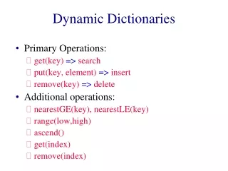
1. Dynamic Dictionaries • Primary Operations: • Get(key) => search • Insert(key, element) => insert • Delete(key) => delete • Additional operations: • Ascend() • Get(index) • Delete(index)

2. n is number of elements in dictionary Complexity Of Dictionary OperationsGet(), Insert() and Delete()

3. D is number of buckets Complexity Of Other OperationsAscend(), Get(index), Delete(index)

4. AVL Tree • binary tree • for every node x, define its balance factor balance factor of x = height of left subtree of x – height of right subtree of x • balance factor of every node x is – 1, 0, or 1

5. -1 Balance Factors 1 1 -1 0 1 0 This is an AVL tree. 0 -1 0 0 0 0

6. Height Of An AVL Tree The height of an AVL tree that has n nodes is at most 1.44 log2 (n+2). The height of every n node binary tree is at least log2 (n+1). log2 (n+1) <= height <=1.44 log2 (n+2)

7. Proof Of Upper Bound On Height • Let Nh = min # of nodes in an AVL tree whose height is h. • N0 = 0. • N1 = 1.

8. L R Nh, h > 1 • Both L and R are AVL trees. • The height of one is h-1. • The height of the other is h-2. • The subtree whose height is h-1 has Nh-1nodes. • The subtree whose height is h-2 has Nh-2nodes. • So, Nh =Nh-1 + Nh-2 + 1.

9. Fibonacci Numbers • F0 = 0, F1 = 1. • Fi =Fi-1 + Fi-2 , i > 1. • N0 = 0, N1 = 1. • Nh =Nh-1 + Nh-2 + 1, i > 1. • Nh =Fh+2 – 1. • Fi ~ fi/sqrt(5). • f = (1 + sqrt(5))/2.

10. -1 10 1 1 7 40 -1 0 1 0 45 3 8 30 0 -1 0 0 0 60 35 1 20 5 0 25 AVL Search Tree

11. Insert(9) -1 10 0 1 1 7 40 -1 0 1 -1 0 45 3 8 30 0 -1 0 0 0 0 60 35 1 9 20 5 0 25

12. -1 Insert(29) 10 1 1 7 40 -1 0 1 0 45 3 8 30 0 -1 0 0 0 -2 60 35 1 20 5 0 -1 RR imbalance => new node is in right subtree of right subtree of white node (node with bf = –2) 25 0 29

13. -1 Insert(29) 10 1 1 7 40 -1 0 1 0 45 3 8 30 0 0 0 0 0 60 35 1 25 5 0 0 20 29 RR rotation.

14. Insert • Following insert, retrace path towards root and adjust balance factors as needed. • Stop when you reach a node whose balance factor becomes 0, 2, or –2, or when you reach the root. • The new tree is not an AVL tree only if you reach a node whose balance factor is either 2 or –2. • In this case, we say the tree has become unbalanced.

15. A-Node • Let A be the nearest ancestor of the newly inserted node whose balance factor becomes +2 or –2 following the insert. • Balance factor of nodes between new node and A is 0 before insertion.

16. Imbalance Types • RR … newly inserted node is in the right subtree of the right subtree of A. • LL … left subtree of left subtree of A. • RL… left subtree of right subtree of A. • LR… right subtree of left subtree of A.

17. A 1 A B B’L B 0 AR B AR A h h h+1 BL BR B’L BR BR AR h h h+1 h h h Before insertion. After insertion. LL Rotation 2 0 • Subtree height is unchanged. • No further adjustments to be done. 1 0 After rotation.

18. A 1 A C B 0 B A B C Before insertion. After insertion. LR Rotation (case 1) 2 0 • Subtree height is unchanged. • No further adjustments to be done. -1 0 0 0 After rotation.

19. A A 1 C B AR B A B 0 AR h h BL BL 0 C BL C’L CR AR C h h h h h-1 h C’L CR CL CR h h-1 h-1 h-1 LR Rotation (case 2) 2 0 • Subtree height is unchanged. • No further adjustments to be done. -1 0 -1 1

20. A 2 A 1 C 0 B -1 AR B A B 0 AR 1 0 h h BL -1 BL 0 C BL CL C’R AR C h h h h-1 h h CL C’R CL CR h-1 h h-1 h-1 LR Rotation (case 3) • Subtree height is unchanged. • No further adjustments to be done.

21. Single & Double Rotations • Single • LL and RR • Double • LR and RL • LR is RR followed by LL • RL is LL followed by RR

22. A 2 A 2 C 0 C AR B -1 AR B A 1 0 h h BL -1 C’R B C BL CL C’R AR h h h h-1 h h BL CL CL C’R h h-1 h-1 h After insertion. After RR rotation. After LL rotation. LR Is RR + LL

23. -1 10 1 1 7 40 -1 0 1 0 45 3 8 30 0 -1 0 0 0 60 35 1 20 5 0 25 Delete An Element Delete 8.

24. -1 10 2 1 7 40 -1 0 1 45 3 30 0 -1 0 0 0 60 35 1 20 5 0 25 Delete An Element q • Let q be parent of deleted node. • Retrace path from q towards root.

25. q New Balance Factor Of q • Deletion from left subtree of q => bf--. • Deletion from right subtree of q => bf++. • New balance factor = 1 or –1 => no change in height of subtree rooted at q. • New balance factor = 0=> height of subtree rooted at q has decreased by 1. • New balance factor = 2 or –2 => tree is unbalanced at q.

26. Imbalance Classification • Let A be the nearest ancestor of the deleted node whose balance factor has become 2 or –2 following a deletion. • Deletion from left subtree of A => type L. • Deletion from right subtree of A => type R. • Type R => new bf(A) = 2. • So, old bf(A) = 1. • So, A has a left child B. • bf(B) = 0 => R0. • bf(B) = 1 => R1. • bf(B) = –1 => R-1.

27. A 1 A 2 B -1 BL B 0 AR B 0 A’R A 1 h h-1 h BL BR BL BR BR A’R h h h h h h-1 Before deletion. After deletion. After rotation. R0 Rotation • Subtree height is unchanged. • No further adjustments to be done. • Similar to LL rotation.

28. A 1 A 2 B 0 BL B 1 AR B 1 A’R A 0 h h-1 h BL BR BL BR BR A’R h h-1 h h-1 h-1 h-1 Before deletion. After deletion. After rotation. R1 Rotation • Subtree height is reduced by 1. • Must continue on path to root. • Similar to LL and R0 rotations.

29. A 2 A 1 C 0 B -1 A’R B A B -1 AR h h-1 BL b BL b C BL CL CR A’R C h-1 h-1 h-1 h-1 CL CR CL CR R-1 Rotation • New balance factor of A and B depends on b. • Subtree height is reduced by 1. • Must continue on path to root. • Similar to LR.

30. Number Of Rebalancing Rotations • At most 1 for an insert. • O(log n) for a delete.

31. Rotation Frequency • Insert random numbers. • No rotation … 53.4% (approx). • LL/RR … 23.3% (approx). • LR/RL … 23.2% (approx).