Download
1 / 14
140 likes | 236 Views
Explore the intricacies of the Normal Distribution in statistics, a symmetrical bell curve representing probabilities for various outcomes. Learn how to calculate probabilities and use standard deviations effectively.

E N D
Probability • Normal Distribution
What is Normal Distribution? • Any event can have at least one possible outcome. • A trialis a single event. An experiment consists of the same trial being performed repeatedly under the same conditions. • If an experiment is performed with enough trials, the populations of each possible outcome can be distributed according to different patterns. this is a typical Poisson Distribution. Note the lack of symmetry. We’re not studying them. This is the symmetrical Gaussian, or Normal Distribution. Learn this! notice the numbers. We’ll deal with them later
How it works... • The Normal Distribution is characterised by grouped continuous data. • The typical graph is a histogram of the populations of each grouped range of possible outcome values For example, if we returned to the era of norm-standardised testing for NCEA, then the distribution of test scores, as percentages, would look something like this: To pass, you would need a score of 50% or greater. Notice about 50% of all candidates achieved this score.
that 50% pass-rate is quite important. • For any Normally-Distributed data, the central peak is the mean, μ. • AND • 50% of all data is <μ; • which means 50% of all data is >μ
a quick bit of revision... • the standard deviation now comes into its own. • Recall: • For a set of continuous data, the mean, μ, is a measure of central tendancy - it is one value that represents the peak data value population. The majority of the data does not equalμ. • The standard deviation, σ, is analogous to the mean difference of every data value from μ. and now, back to the graph and it’s numbers...
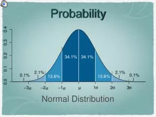
features of Normal Distribution... the x-axis is asymptotic 68% of all data lie within 1σ of μ 95% of all data lie within 2σ of μ 99% of all data lie within 3σ of μ the peak is the mean, μ. 50% of the data lie either side of μ. the distribution is symmetrical about μ
summary: • the x-axis is asymptotic • the peak is the mean, μ. • the distribution is symmetrical about μ; 50% of the data lie either side of μ. • 68% of all data lie within 1σ of μ • 95% of all data lie within 2σ of μ • 99% of all data lie within 3σ of μ } these percentages are rounded this distribution lets us calculate the probability that any outcome will be within a specified range of values
X - μ σ Z = Ah, the wonder that is u Z • The Normal Distribution of outcome frequencies is defined in terms of how many standard deviations either side of the mean contain a specified range of outcome values. • In order to calculate the probability that the outcome of a random event X will lie within a specified multiple of σ either side of μ, we use an intermediate Random Variable, Z. For this relationship to hold true, for Z, σ = 1 and μ = 0; hence, for a Normally distributed population, the range is from -3σ to +3σ
Z, PQR, and You • Probability calculations using Z give the likelihood that an outcome will be within a specified multiple of σ from the mean. There are three models used: P(t) = the probability that an outcome t is any value of X up to a defined multiple of σ beyond μ P(Z<t) ≡ P(μ<Z<t) + 0.5 Q(t) = the probability that an outcome t is any value of X between μ and a defined multiple of σ P(μ<Z<t) R(t) = the probability that an outcome t is any value of X greater than a defined multiple of σ below μ P(Z>t)
Solving PQR Problems • Enter RUN mode. • OPTN • F6 • F3 • F6 • Read the problem carefully. • Draw a diagram - sketch the Bell Curve, and use this to identify the problem as P, Q or R • You could now use the Z probability tables to calculate P, Q or R, or use a Graphic Calculator such as the Casio fx-9750G Plus This gives the F-menu for PQR. 1. Choose the function (P, Q or R) appropriate to your problem; 2. enter the value of t, and EXE.
[ ] SO... use to calculate Z, and then use PQR. X - μ σ [ ] Z = 20-μ σ 20-33 8 P(X<20) = P(Z < ) = P(Z < ) Calculating Z from Real Data The PQR function assumes a perfectly-symmetrical distribution about μ. Real survey distributions are rarely perfect. For any set of real data, we can calculate μ and σ, and therefore Z. For example, if μ=33 and σ=8, then to find P(X<20): = P(Z < -1.625) Now, use the R function, and subtract the result from 1.
X = Z σ + μ Inverse Normal • This is the reverse process to finding the probability. • Given the probability that an event’s outcome will lie within a defined range, we can rearrange the Z equation to give But... we cannot define X, as it represents the entire range of values of all possible outcomes. What the equation will give us is the value k. k is the upper or lower limit of the range of X that is included in the P calculations
an example... • if X is a normally-distributed variable with • σ=4, μ=25, and p(X<k) = 0.982, what is k? The long way... • using a graphic calculator, for example the trusty Casio fx9750G; • MODE: STATS • F5 ➜ F1 ➜ F3 • Area = probability, as a decimal • σ = • μ = • EXECUTE Use the PQR model, and sketch a bell curve to identify the regions being included in the p range. Use the ND table to find the value of Z: Z range is from -1 to +1, so find 0.982 - 0.5 = 0.482 Gives Z = 2.097 So, k = 4 x 2.097 + 25 = 33.388 or, the short way...
next lesson... • confidence intervals


