Download
1 / 59
590 likes | 837 Views
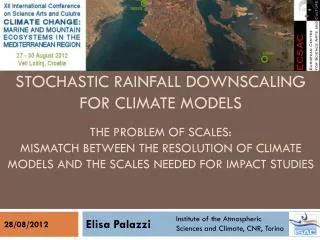
Stochastic rainfall downscaling FOR climate models The problem of scales : Mismatch between the resoluTIon of climate models and the scales needed for impact studieS. Elisa Palazzi. 28/08/2012. Institute of the Atmospheric Sciences and Climate , CNR, Torino.

E N D
Stochastic rainfall downscaling FOR climate modelsThe problemofscales: Mismatchbetween the resoluTIonofclimatemodels and the scalesneededfor impact studieS Elisa Palazzi 28/08/2012 Instituteof the AtmosphericSciences and Climate, CNR, Torino
Introduction & outline • Precipitation is a key component of the hydrological cycle and one of the most important parameters for a range of natural and socioeconomic systems. The study of consequences of global climate change on these systems requires scenarios of future precipitation change at the local scale as input to impact models. • Direct application of output from GCMs and RCMs is inadequate because of the coarse spatial resolution and limited representation of mesoscale atmospheric processes, topography, and land-sea distribution. • Of particular concern with precipitation, GCMs exhibit a much larger spatial scale than is usually needed in impact studies and this leads to inconsistencies in rainfall statistics, extremes and small-scale variability, particularly in the presence of complex terrain and heterogeneous orography.
Introduction & outline • Techniques have been developed to downscale information from GCMs (RCMs) to regional (local) scales. (Dynamical, statistical and stochastic downscaling) • In the absence of full deterministic modelling of small-scale rainfall, stochastic downscaling techniques generate ensembles of possible realizations of small scale rainfall fields starting from a smoother distribution on larger scale. • Small scale fields are consistent with the large scale features of the coarse field and the known statistical properties of the small-scale rainfall fields. • Stochastic downscaling is not a substitute for physically-based dynamical models, also used to better understand rainfall dynamics; it is a way to introduce variability at scales not resolved by physical models.
Modellingchain: bridging the gap • Global Climate Models • Global Reanalyses 100-120 km Dynamical downscaling 10-30 km Regional Climate Models hydrostatic non-hydrostatic Stochastic downscaling High-resolution Climate Scenarios few km Hydrological models Rainfall-runoff models Model-measurement comparison Future projections of water availability Flood forecasting , etc.
GCMs ~ 500 km • The most advanced tools currently available for simulating the global climate system (physical processes in the atmosphere, ocean, cryosphere and land surface, and their interactions) and the response of the global climate system to anthropogenic and natural forcings. • Spatial Resolution: 100-120 km ~ 110 km • GCMsspatial resolution is too coarse to capture the local aspects (smooth topography)and it is limited by computational resources. • The sub-grid physical processes have to be parameterized. Parameterization is a way of describing the aggregated effect of sub-grid processes over a larger scale. • Parameterization is one source of uncertainty in simulations of current/future climate.
An important field: Rainfall • Highly non-homogeneous phenomenon • Phenomenon organized in hierarchic structures (scaling property of rainfall) • Convective scale (or microscale) 0-20 km • (convective cells characterized by high precipitation intensity and short duration) embedded within • Mesoscale20-200 km (clusters of lower precipitation intensity) embedded within • Synoptic scale > 1000 km • (scale of the general circulation) • - Highly intermittent in space and time (alternating between dry and rainy periods). convectivecells mesoscalestructures Synoptic scale No interpolation (nearest neighbors, linear interpolation, distance-weighted interpolation) is possible.
Needfordownscaling • - Climatemodelsimulations/predictionsneedtobegenerated at finerscalesthanthoseofGCMsiftheirresults are tobeofuse • The need is for regional climate scenarios but the most complete models are the coupled GCMs • 1) One solution is to employ EMICs, developed to emphasize particular aspects of the climate system. • 2) Another is to run the full GCM at a finerresolution(or enhancedresolution in the regionsof interest). Thiswouldrequire a verypowerful computer (suchas the Earth Simulator in Japan) or a very short simulationperiod (timeslice, e.g. 5years)
Downscaling - generating locally relevant data from GCMs. 3) Another is to downscale climate data: a strategy for generating locally relevant data from GCMs. Downscaling can be done in several ways. Three categories: - Dynamical downscaling - Statistical downscaling - Stochastic downscaling
Dynamical Downscaling Nesting a RCM into an existing GCM. RCMs work by increasing the resolution of the GCM in a limited area (e.g., the size of western Europe, or southern Africa). They need the climate (temperature, wind etc.) calculated by the GCM as boundary conditions (large scale driving factors) for the regional simulation. RCMs can represent the effects of mountains, coastlines, changing vegetation characteristics on the weather much better than GCMs. They can provide weather and climate information at resolutions as fine as 50 km to 20 km. WRF, RAMS, ROMS, COSMO-CLM, PROTHEUS, RegCM, etc.
Dynamical Downscaling • RCMs vs GCMs • simulate/predictclimate/climatechanges more realistically, with more detail and withregionaldifferences • are muchbetter at simulating and predictingchangestoextremesofweather Predictedchanges in winterprecipitationoverEuropebetween the presentday and 2080. Largereductionsover the Alps and Pyrenees are predictedby the RCM (right), butnot the GCM (left)
StatisticalDownscaling Use of statistical regressions. These techniques assume that the relationship between large scale climate variables (e.g. grid box rainfall and pressure) and the actual rainfall measured at one particular raingauge will always be the same. So, if that relationship is known for current climate, the GCM projections of future climate can be used to predict how the rainfall measured at that raingauge will change in the future. Wilby et al, WRR 1998
StochasticDownscaling • Generates stochastic ensembles of small-scale predictions from the output of atmospheric models or from a measured field with a coarse spatial or temporal resolution, using different approaches, e.g.: • Random distribution of rain cells • Multifractal cascades based on the theory of scaling in rainfall • Nonlinearly transformed spectral models • (Ferraris et al., 2003 – comparison of the various methods and their skill) • Suitable for precipitation • The precipitation fields generated by stochastic procedures are consistent with the large-scale features imposed by meteorological forecast, as the total rainfall volume, and with the known statistical properties of precipitation at multiple scales.
RainFARM procedure Rebora et al., J. Hydrometeorol., 2006 • RainfallFiltered Auto Regressive Model (RainFARM) • It belongs to the family of “Metagaussian models”, based on nonlinearly filtering the output of a linear autoregressive process, whose properties are derived from the information available at the large scales. • Extrapolates the large-scale spatio-temporal power spectrum of the meteorological predictions to the small, unresolved scales. The basic idea is to preserve amplitude and phases of the original field at the scales at which we are confident in the limited area meteorological model prediction and to reconstruct the Fourier spectrum at the smaller (unreliable, unresolved) scales. • It is able to reproduce the small-scale statistics of the precipitation – scaling properties of the main statistical moments, spatiotemporal correlation structure of the fields, etc. – and capture the temporal persistence of the observed precipitation at the scales smaller than the reliability scales.
RainFARM procedure in detail Input field (model output) Fourier spectrum • Space-timepowerspectrum (assume a power low form), and estimate or fix the spectralslopesa, b ; ; Fourier and powerspectrumextrapolated at lowerscales, withrandomphases (f) g: gaussianfieldobtainedbyinverting Syntheticprecipitationfield, obtainedby a nonlineartranformationofg
RainFARM procedure in detail Toforce the output fieldrtbeequaltoP on scaledlargerthan the confidencescales, wecoarse-grain the field L0 , T0 Finally, weobtain the output of the downscaling procedure, r, withresolutionl and t, byimposing: r = P, aggregating on L0 , T0 The stochastic nature of the downscaled field, r, is associated with the choice of a set of random Fourier phases (different phases different realizations)
RainFARM - summary • Purpose • to generate a stochastic precipitation field, r • starting from a larger-scale field, P, reliable at the scales L0 and T0 (the only free parameters of the method) • such that aggregating r on L0 and T0 give a coarse-grained field R; R=P r is modelled in terms of a nonlinear (static) transformation of a linear autoregressive process r (output)= one stochastic realization of the smmal-scale precipitation field l, t= spatial and temporal scales (l << L0 , t << T0 ) P (input) = predicted or measured large-scale precipitation field L0, T0 = reliable spatial and temporal scales
Test on RainFARM • Coarsegraining (degradation) of a high-resolutionmeasuredprecipitationfield, p • pobtainedfrom radar measurements at San Pietro Capofiume, Emilia Romagna, Italy (ARPA-SIM data). • Eventof 25 December 2001, starting at 0000 UTC. • Data resolution: 1km, 15 min. • Maximumscales:128 km, 16 h • Coarse-graining 8km, 1h. • Generation of a smootherfield, P, usedas the input to the downscalingmodel. Generation of the downscaledfield, r • Performance of the downscaling procedure verifiedbyassessingwhether the reconstructedfieldsrreproduce the correctrainfall pattern and the statisticalpropertiesof the truefield p.
Test on RainFARM Rebora et al., 2006 RainFARM ensemble (95%) RainFARMens. mean Original Timeevolutionof the instantaneousspatialaverageof the originalfieldp and ofan ensemble of 100 realizationsof the stochasticfieldr(x, y, t) producedbyRainFARM (for a midlatitude intense rainfallevent).
Test on RainFARM Rebora et al., 2006 Temporalpowerspectrum Spatialpowerspectrum Spatial and temporalpowerspectraof the originalfieldp(x, y, t) and an ensemble of 100 realizationsof the stochasticfieldr(x, y, t) producedbyRainFARM
Test on RainFARM Rebora et al., 2006 Statisticalmoments
RainFARMapplications Spatio-temporaldownscalingof intense rainfallevents and operationalapplications (e.g., forecastingfloodsin smallcatchments) (Rebora et al., 2005,2006) Stochasticdownscalingas a methodtoquantitatively compare numericalforecasts and raingaugemeasurements and verifylimited-areamodelpredictionskills (e.g., Brussolo et al., 2008) Climatic and climate change studies: downscaling of GCM and RCM outputs and generation of high-resolution precipitation fields for present and future conditions (Variant of RainFARM for purely spatial downscaling) examples of application to the PROTHEUS (case 1) and COSMO-CLM (case 2) regional models
B.Verificationofrainfallforecast via stochasticdownscaling Usually, the verification of meteorological forecasts (e.g., for assessment of hydrological risk) is made through comparison with different observational sources (e.g., raingauge data), by 1- upscaling rain gauge data limited representativeness and large uncertainities 2- downscaling the model output to the gauge positions underestimation of the local precipitation variability Brussolo et al., 2008: RainFARMusedtodownscalenumericalprecipitationforecasts (COSMO-LAMI model): 50 high resolution (1h, 850 m) stochasticrealizationsforeachmodelforecast and comparisonwithraingauge data accumulatedover 1-h period. Oneadvantageisthatensemblesofstochasticfields can beusedtocharacterize the expectedvariability at eachraingauge position
B.Verificationofrainfallforecast via stochasticdownscaling Brussolo et al., 2008
C.ClimaticApplication– case 1 • Global Climate Models • Global Reanalyses ERA40 Dynamical downscaling Regional Climate Models PROTHEUS Stochastic downscaling High-resolution Climate Scenarios RainFarm Modelprecipitation vs data from a raingauge network in the Piedmont and Val d’Aosta regions, Italy Model-measurement comparison
Aim Is the precipitation produced by the PROTHEUS RCM and spatially downscaled stochastically with the RainFARM procedure able to reproduce the main statistical properties of precipitation observed by a network of rain gauges?
Approach PROTHEUS vs rain-gauge data averaged in the modelpixels PROTHEUS vs individualrain-gauge data Downscaled PROTHEUS vs individualrain-gauge data 1 Beforedownscaling 2 3 Afterdownscaling Analysis on annual and seasonalbasisof: - Timeseriesof total precipitation - PDFsof total precipitation - PDFsofprecipitationintensity - PDFsofno-rain and rainyperiods - Numberofdayswith no rain.
PROTHEUS RegionalClimateModel Atmosphere-ocean RCM for the Mediterraneanbasin utmea.enea.it/research/PROTHEUS/ ATMOSPHERIC MODEL 30 km res. COUPLER OCEANIC MODEL Artaleet al., ClimateResearch, 2012
PROTHEUS RegionalClimateModel • Large scale driver: ERA40 • Domain usedforthisstudy: • (5.5°E-11.5°E, 43°N-47.3°N) Cumulatedannualprecipitation Artaleet al., ClimateResearch, 2012
Rain-gauge network Average station altitude [m] • 122 raingauges • 1958-2001 • Altitudemax: 2526 m • Altitude min: 127 m • Dailyresolution • Raingaugesnotuniformlydistributed in the 33 modelpixels • Mininum (maximum) numberofstations per pixel = 1 (11)
PROTHEUS vs aggregated raingauges 1 Timeseries r= 0.8 Monthlycorrelation SON MAM JJA PROTHEUS Raingauges The interannualvariabilityof PROTHEUS reflectsthatof the forcing field (ERA40)
PROTHEUS vs aggregated raingauges 1 Spatialdistributionof the correlationcoefficient Relatedto the numberofraingauges per pixel 0.4 < c < 0.8
PROTHEUS vs aggregated raingauges 1 Spatiallyaveragedoverallmodelpixels (alsotrueforeach pixel) Averageof total precipitation Numberof “zeros” (dry days) Averageofprecipitationintensity p0 = 0.1 mm/day The modeldoesnot produce more rainthan the observations, butrain in the modelis more frequent.
PROTHEUS vs aggregatedraingauges GOOD 1 LESS GOOD PDFsof total precipitation YEAR PROTHEUS Raingauges N0_model = 47% N0_obs = 64% P0= 0.1 mm/day
PROTHEUS vs individualraingauges GOOD 2 LESS GOOD YEAR PROTHEUS Raingauges
PROTHEUS vs individualraingauges GOOD 2 LESS GOOD NEED FOR DOWNSCALING! YEAR PROTHEUS Raingauges
RainFARMdownscaling: example Example SON 1958 30 km ~ 1 km Precipitationfieldfrom PROTHEUS Stochasticrealizationof the PROTHEUS downscaledfield, obtainedwithRainFARM
PROTHEUS downscaled vs individualraingauges GOOD 3 LESS GOOD YEAR PROTHEUS Raingauges N0_model = 47% (70%) N0_obs = 72% P0= 0.1 (2) mm/day
Numberofzeros Thresholdfor zero rain: p0=0.1 mm/day “Upscaling” “Downscaling” Almost the same: the downscaling procedure is not able to correct the number of zeros P0 (model)= 2 mm/day improves the comparison 72 %(obs) vs 70% (mod)
Summary case 1 • The averageprecipitationof PROTHEUS data has a high bias. Thereis a strong biasalso in the numberof dry dayswhichislowerfor the model (47%) thanfor the obs. (64%), using a thresholdof 0.1 mm/day. Thereis a strong correlationbetween the interannualvariabilityofmodel data (reflectingthatof the large scale driver) and observed data. BEFORE DOWSCALING • Comparisonbetween PROTHEUS and the rain-gauge data AVERAGED in the modelpixels: The PDFsfrommodel and the obs. agreewell (except in winter). • Comparisonbetween PROTHEUS and data fromindividualraingauges: the PDFs do notagreewell, rain-gauge data show much more extremeevents, notcapturedby the model AFTER DOWSCALING • Comparisonbetween PROTHEUS (downscaledwithRainFARM) and data fromindividualraingauges: the PDF agreement improves (except in winter). The numberof dry daysremainverydifferent in the model and the observations. Using a no-rainthresholdof2 mm/dayfor the model, the modelcapturesverywell the numberof dry days.
Summary case 1 • The stochasticdownscaling procedure cannotcorrect the modeloutputs at large scale, suchas the disagreement in the frequencyofprecipitationevents, particularlyevidentduring the winterseason • The high-resolutionprecipitationfieldsobtainedbydownscaling the PROTHEUS output reproducewell the seasonality and the amplitudedistributionof the observedraingaugeprecipitationduringmostof the year.
C.ClimaticApplication– case 2 • Global Climate Models • Global Reanalyses CMCC-MED 80 km Dynamical downscaling Regional Climate Models COSMO-CLM 8 km Stochastic downscaling High-resolution Climate Scenarios RainFarm Modelprecipitation vs data fromindividualraingauges in Africa (CLUVA project) Model-measurement comparison
Comparisonbetween COSMO-CLM and groundrainfall data WEST Domain 18°W-15.17°E 3.3 °N-16.8°N 465x190 gridpoints • EAST Domains • 34.4°E-42.9°E • 6.1°N-12.5°N 120x90 gridpoints • - 34.5°E-41.3°E • 11.8°S-2.1°S • 95 x 135 gridpoints St.Louis (16.5 W, 16.03 N)Ougadougou (1.55 W, 12.37 N) Douala (9.71 E, 4.045 N) Addis Abeba (38.75 E, 9.02 N) Dar esSalaam (39.27 E, 6.82 S) 1950-2050
Dar esSalaam and Douala Rainfallannualcycle Dar esSalaam Douala
RainFARMdownscaling: example Example MAM, area of Doula Stochasticrealization of the COSMO-CLM downscaledfield, obtained with RainFARM Precipitationfield from COSMO-CLM
Comparisonbetweendownscaled COSMO-CLM and groundrainfall data Dar esSalaam Douala WHOLE YEAR PDFs
Summary- case 1 Annualrainfallcycle and rainfallPDFs at Dar es Salaam and Douala are onlymarginallyreproducedby COSMO-CLM Stochasticdownscaling of the 8-km COSMO-CLM fieldsdoesnotimprove the agreement with the data
Open questions At smallscales, strong (on-off) intermittencychanges the powerspectrum and PDF shape and functionallaw. PDF PowerSpectrum
Last slide Thanksto Donatella D’Onofrio Jost von Hardenberg Antonello Provenzale ISAC-CNR Vincenzo Artale Sandro Calmanti ENEA-UTMEA and toallofyouforyourattention!