Download
1 / 62
620 likes | 736 Views
Simultaneous estimation of Trees and Alignments, or Complexity and The Tree of Life. Tandy Warnow The University of Texas at Austin. How did life evolve on earth?. An international effort to understand how life evolved on earth

E N D
Simultaneous estimation of Trees and Alignments, orComplexity and The Tree of Life Tandy Warnow The University of Texas at Austin
How did life evolve on earth? An international effort to understand how life evolved on earth Biomedical applications: drug design, protein structure and function prediction, biodiversity. • Courtesy of the Tree of Life project
-3 mil yrs AAGACTT AAGACTT -2 mil yrs AAGGCCT AAGGCCT AAGGCCT AAGGCCT TGGACTT TGGACTT TGGACTT TGGACTT -1 mil yrs AGGGCAT AGGGCAT AGGGCAT TAGCCCT TAGCCCT TAGCCCT AGCACTT AGCACTT AGCACTT today AGGGCAT TAGCCCA TAGACTT AGCACAA AGCGCTT AGGGCAT TAGCCCA TAGACTT AGCACAA AGCGCTT DNA Sequence Evolution
U V W X Y AGGGCAT TAGCCCA TAGACTT TGCACAA TGCGCTT X U Y V W
Local optimum Cost Global optimum Phylogenetic trees Phylogenetic reconstruction methods • Hill-climbing heuristics for hard optimization criteria (Maximum Parsimony and Maximum Likelihood) • Polynomial time distance-based methods, e.g. Neighbor Joining, FastME, UPGMA, etc. • Bayesian MCMC methods
Solving NP-hard problems exactly is … unlikely • Number of (unrooted) binary trees on n leaves is (2n-5)!! • If each tree on 1000 taxa could be analyzed in 0.001 seconds, we would find the best tree in 2890 millennia
Standard Markov models • Sequences evolve just with substitutions • Sites (i.e., positions) evolve i.i.d. (identically and independently), and have “rates of evolution” that are drawn from a common distribution (typically gamma) • Numerical parameters describe the probability of substitutions of each type on each edge of the tree
Jukes-Cantor (simplest DNA model) • DNA sequences (A,C,T,G) evolve just with substitutions • Sites (i.e., positions) evolve i.i.d. (identically and independently) • If a site changes on an edge, it changes with equal probability to the remaining states (A,C,G,T) • Numerical parameters p(e): for each edge in the tree, p(e) denotes the probability that each site changes on e A Jukes-Cantor model tree is a pair (T,), where T is a tree and denotes the numerical parameters p(e), one for each edge e in the tree T. Note that the JC model is time-reversible, so that without an assumption of the molecular clock, the root cannot be identified, even given infinite data
Questions • Statistical consistency: Is the given phylogeny reconstruction method guaranteed to reconstruct the model tree when infinitely long sequences are available? • Convergence rate (sample size complexity): How long do the sequences need to be for the method to be accurate with high probability? • Identifiability: Is the model tree uniquely identified by the “pattern probabilities” (i.e., by infinitely long sequences)?
Quantifying Error FN FN: false negative (missing edge) FP: false positive (incorrect edge) 50% error rate FP
Statistical consistency, exponential convergence, and absolute fast convergence (afc)
Current state of knowledge (for substitution-only models) • We have established much of the statistical performance (consistency and convergence rates) of the major methods for phylogeny estimation. • We have developed “fast converging” methods (guaranteed to reconstruct the true tree from polynomial length sequences) with excellent performance in practice. • We have very fast methods for solving maximum likelihood and maximum parsimony, the major optimization problems, even for large datasets.
Neighbor Joining’s sequence length requirement is exponential! • Atteson: Let T be a General Markov model tree defining distance matrix D. Then Neighbor Joining will reconstruct the true tree with high probability from sequences that are of length at least O(lg n emax Dij), where n is the number of leaves in T.
Neighbor joining has poor performance on large diameter trees [Nakhleh et al. ISMB 2001] Simulation study based upon fixed edge lengths, K2P model of evolution, sequence lengths fixed to 1000 nucleotides. Error rates reflect proportion of incorrect edges in inferred trees. 0.8 NJ 0.6 Error Rate 0.4 0.2 0 0 400 800 1200 1600 No. Taxa
DCM1-boosting distance-based methods[Nakhleh et al. ISMB 2001] • Theorem: DCM1-NJ converges to the true tree from polynomial length sequences 0.8 NJ DCM1-NJ 0.6 Error Rate 0.4 0.2 0 0 400 800 1200 1600 No. Taxa
Maximum Likelihood (ML) • Given: Set S of aligned DNA sequences, and a parametric model of sequence evolution (e.g., Jukes-Cantor) • Objective: Find model tree (T,) to maximize Pr[S|T,]. Statistically consistent, but not known to be afc (best upper bound on sequence length requirement is exponential) NP-hard Excellent heuristics exist (e.g., RAxML) that produce highly accurate trees
Maximum Likelihood (ML) • Given: Set S of aligned DNA sequences, and a parametric model of sequence evolution (e.g., Jukes-Cantor) • Objective: Find model tree (T,) to maximize Pr[S|T,]. Statistically consistent, but not known to be afc (best upper bound on sequence length requirement is exponential) NP-hard Excellent heuristics exist (e.g., RAxML) that produce highly accurate trees
Much mathematical theory about convergence rates for phylogeny estimation methods Fast-converging polynomial time distance-based methods with excellent performance in simulation (DCM1-NJ and others). Maximum likelihood: statistically consistent, with excellent heuristics, producing highly accurate trees (established using simulations) on large datasets Is phylogeny estimation Solved?
Much mathematical theory about convergence rates for phylogeny estimation methods Fast-converging polynomial time distance-based methods with excellent performance in simulation (DCM1-NJ and others). Maximum likelihood: statistically consistent, with excellent heuristics, producing highly accurate trees (established using simulations) on large datasets Is phylogeny estimation Solved?
Much mathematical theory about convergence rates for phylogeny estimation methods Fast-converging polynomial time distance-based methods with excellent performance in simulation (DCM1-NJ and others). Maximum likelihood: statistically consistent, with excellent heuristics, producing highly accurate trees (established using simulations) on large datasets Is phylogeny estimation Solved?
Much mathematical theory about convergence rates for phylogeny estimation methods Fast-converging polynomial time distance-based methods with excellent performance in simulation (DCM1-NJ and others). Maximum likelihood: statistically consistent, with excellent heuristics, producing highly accurate trees (established using simulations) on large datasets Is phylogeny estimation Solved?
No, because standard Markov models are too simple! Simplifying assumptions: • Sequences evolve just with substitutions • Sites (i.e., positions) evolve identically and independently, and have “rates of evolution” that are drawn from a common distribution (typically gamma)
No, because standard Markov models are too simple! Simplifying assumptions: • Sequences evolve just with substitutions • Sites (i.e., positions) evolve identically and independently, and have “rates of evolution” that are drawn from a common distribution (typically gamma)
indels (insertions and deletions) also occur! Deletion Mutation …ACGGTGCAGTTACCA… …ACCAGTCACCA…
Deletion Mutation The true pairwise alignment is: …ACGGTGCAGTTACCA… …AC----CAGTCACCA… …ACGGTGCAGTTACCA… …ACCAGTCACCA… The true multiple alignment on a set of homologous sequences is obtained by tracing their evolutionary history, and extending the pairwise alignments on the edges to a multiple alignment on the leaf sequences.
Input: unaligned sequences S1 = AGGCTATCACCTGACCTCCA S2 = TAGCTATCACGACCGC S3 = TAGCTGACCGC S4 = TCACGACCGACA
Phase 1: Multiple Sequence Alignment S1 = AGGCTATCACCTGACCTCCA S2 = TAGCTATCACGACCGC S3 = TAGCTGACCGC S4 = TCACGACCGACA S1 = -AGGCTATCACCTGACCTCCA S2 = TAG-CTATCAC--GACCGC-- S3 = TAG-CT-------GACCGC-- S4 = -------TCAC--GACCGACA
Phase 2: Construct tree S1 = AGGCTATCACCTGACCTCCA S2 = TAGCTATCACGACCGC S3 = TAGCTGACCGC S4 = TCACGACCGACA S1 = -AGGCTATCACCTGACCTCCA S2 = TAG-CTATCAC--GACCGC-- S3 = TAG-CT-------GACCGC-- S4 = -------TCAC--GACCGACA S1 S2 S4 S3
Phylogeny methods Maximum likelihood Bayesian MCMC Maximum parsimony Neighbor joining FastME UPGMA Quartet puzzling Etc. Many methods Alignment methods • Clustal • POY (and POY*) • Probcons (and Probtree) • MAFFT • Prank • Muscle • Di-align • T-Coffee • Opal • Etc. RAxML: best heuristic for large-scale ML optimization
S1 S1 S2 S4 S4 S2 S3 S3 Simulation Studies S1 = AGGCTATCACCTGACCTCCA S2 = TAGCTATCACGACCGC S3 = TAGCTGACCGC S4 = TCACGACCGACA Unaligned Sequences S1 = -AGGCTATCACCTGACCTCCA S2 = TAG-CTATCAC--GACCGC-- S3 = TAG-CT-------GACCGC-- S4 = -------TCAC--GACCGACA S1 = -AGGCTATCACCTGACCTCCA S2 = TAG-CTATCAC--GACCGC-- S3 = TAG-C--T-----GACCGC-- S4 = T---C-A-CGACCGA----CA Compare True tree and alignment Estimated tree and alignment
Problems with the two-phase approach • Current alignment methods fail to return reasonable alignments on large datasets with high rates of indels and substitutions. • Manual alignment is time consuming and subjective. • Systematists discard potentially useful markers if they are difficult to align. This issues seriously impact large-scale phylogeny estimation (and Tree of Life projects)
S1 S2 S4 S3 S1 = AGGCTATCACCTGACCTCCA S2 = TAGCTATCACGACCGC S3 = TAGCTGACCGC S4 = TCACGACCGACA and S1 = -AGGCTATCACCTGACCTCCA S2 = TAG-CTATCAC--GACCGC-- S3 = TAG-CT-------GACCGC-- S4 = -------TCAC--GACCGACA Statistical simultaneous estimation methods (BALiPhy, Alifritz, Statalign) are not scalable. POY and related methods are not more accurate than standard two-phase methods.
SATé: (Simultaneous Alignment and Tree Estimation) • Liu, Nelesen, Raghavan, Linder, and Warnow • Search strategy: search through tree space, and realigns sequences on each tree using a novel divide-and-conquer approach, attempting to optimize the GTR+Gammamaximum likelihood score. • Software at http://phylo.bio.ku.edu/software/sate/sate.html • Science, 19 June 2009, pp. 1561-1564.
Obtain initial alignment and estimated ML tree Tree SATé Algorithm
Obtain initial alignment and estimated ML tree Tree Use tree to compute new alignment Alignment SATé Algorithm
Obtain initial alignment and estimated ML tree Tree Use tree to compute new alignment Estimate GTR+Gamma ML tree on new alignment Alignment SATé Algorithm
Obtain initial alignment and estimated ML tree Tree Use tree to compute new alignment Estimate GTR+Gamma ML tree on new alignment Alignment SATé Algorithm If new alignment/tree pair has worse GTR+Gamma ML score, realign using a different decomposition Repeat until termination condition (typically, 24 hours)
1000 taxon models, ordered by difficulty 24 hour SATé analysis, on desktop machines (Similar improvements for biological datasets)
Why is SATé so accurate? • Not because it’s good to optimize ML under a model treating gaps as missing data - we prove that this optimization problem is a bad approach.
Extended Jukes-Cantor model • Sites evolve i.i.d • The state at the root is random • Substitution probabilities p(e) on each edge e satisfy 0 ≤ p(e) < 3/4. • If a substitution occurs on an edge e, the nucleotide changes to the remaining nucleotides with equal probability.
Negative result • Let S be a set of DNA sequences, and let Opt(S)= max Pr[A|T,], where A is an alignment on S and (T,) is an EJC model tree for S. • Let BestTrees(S)={T: for some and some alignment A, Pr[A|T,]=Opt(S)} • Theorem: For all sets S of unaligned DNA sequences, BestTrees(S) contains all trees on S.
Why is SATé so accurate? • Not because it’s good to optimize ML under GTR+Gamma • Instead, the key is the divide-and-conquer technique used in the re-alignment strategy.
Since the Science paper: SATé-II: • Uses a different re-alignment strategy, but same general algorithm design. • More accurate than SATé and much faster!
SATé-I vs.SATé-II SATé-II • Faster and more accurate than SATé-I • Longer analyses or use of ML to select tree/alignment pair slightly better results
SATé Software • Downloadable software (with user-friendly gui) • Developers: Mark Holder and Jiaye Yu at the University of Kansas • Webpage http://phylo.bio.ku.edu/software/sate/sate.html
Complexity viz. The Tree of Life • Algorithmic complexity (e.g., running time and NP-hardness) • Sample size complexity (e.g. how long do the sequences need to be to obtain a highly accurate reconstruction with high probability?) • Stochastic model complexity (i.e., how realistic are the models of evolution, and what are the consequences of making the models more realistic?)