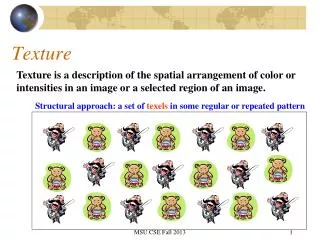
Texture
Texture. Texture. Edge detectors find differences in overall intensity. Average intensity is only simplest difference. many slides from David Jacobs. Issues: 1) Discrimination/Analysis. (Freeman). 2) Synthesis. Other texture applications. 3. Texture boundary detection. Segmentation

Texture
E N D
Presentation Transcript
Texture • Edge detectors find differences in overall intensity. • Average intensity is only simplest difference. many slides from David Jacobs
Issues: 1) Discrimination/Analysis (Freeman)
Other texture applications 3. Texture boundary detection. Segmentation 4. Shape from texture.
Texture gradient associated to converging lines (Gibson1957)
What is texture? • Something that repeats with variation. • Must separate what repeats and what stays the same. • Model as repeated trials of a random process • The probability distribution stays the same. • But each trial is different.
Simplest Texture • Each pixel independent, identically distributed (iid). • Examples: • Region of constant intensity. • Gaussian noise pattern. • Speckled pattern
Texture Discrimination is then Statistics • Two sets of samples. • Do they come from the same random process?
Simplest Texture Discrimination • Compare histograms. • Divide intensities into discrete ranges. • Count how many pixels in each range. 0-25 26-50 51-75 76-100 225-250
How/why to compare • Simplest comparison is SSD, many others. • Can view probabilistically. • Histogram is a set of samples from a probability distribution. • With many samples it approximates distribution. • Test probability samples drawn from same distribution. Ie., is difference greater than expected when two samples come from same distribution?
Chi square distance between texton histograms Chi-square i 0.1 j k 0.8 (Malik)
More Complex Discrimination • Histogram comparison is very limiting • Every pixel is independent. • Everything happens at a tiny scale. • Use output of filters of different scales.
Origin: First-order gray-level statistics: characterized by histogram Second-order gray-level statistics: described by co-occurrence matrix Autocorrelation function I(i,j)*I(-i,-j) Power spectrum of I(i,j) is square of magnitude of Fourier Transform Power spectrum of a function is Fourier transform of autocorrelation Various methods use Fourier transform (in polar representation)
What are Right Filters? • Multi-scale is good, since we don’t know right scale a priori. • Easiest to compare with naïve Bayes: Filter image one: (F1, F2, …) Filter image two: (G1, G2, …) S means image one and two have same texture. Approximate: P(F1,G1,F2,G2, …| S) By P(F1,G1|S)*P(F2,G2|S)*…
What are Right Filters? • The more independent the better. • In an image, output of one filter should be independent of others. • Because our comparison assumes independence. • Wavelets seem to be best.
Gabor Filters Gabor filters at different scales and spatial frequencies top row shows anti-symmetric (or odd) filters, bottom row the symmetric (or even) filters.
Gabor filters are examples of Wavelets • We know two bases for images: • Pixels are localized in space. • Fourier are localized in frequency. • Wavelets are a little of both. • Good for measuring frequency locally.
Markov Model • Captures local dependencies. • Each pixel depends on neighborhood. • Example, 1D first order model P(p1, p2, …pn) = P(p1)*P(p2|p1)*P(p3|p2,p1)*… = P(p1)*P(p2|p1)*P(p3|p2)*P(p4|p3)*…
Markov Chains • Markov Chain • a sequence of random variables • is the state of the model at time t • Markov assumption: each state is dependent only on the previous one • dependency given by a conditional probability: • The above is actually a first-order Markov chain • An N’th-order Markov chain:
A D X B C • Higher order MRF’s have larger neighborhoods * * * * * * * * X * * * X * * * * * * * * * Markov Random Field • A Markov random field (MRF) • generalization of Markov chains to two or more dimensions. • First-order MRF: • probability that pixel X takes a certain value given the values of neighbors A, B, C, and D:
Texture Synthesis [Efros & Leung, ICCV 99] • Can apply 2D version of text synthesis
Synthesizing One Pixel SAMPLE • What is ? • Find all the windows in the image that match the neighborhood • consider only pixels in the neighborhood that are already filled in • To synthesize x • pick one matching window at random • assign x to be the center pixel of that window x sample image Generated image
Really Synthesizing One Pixel SAMPLE x sample image Generated image • An exact neighbourhood match might not be present • So we find the best matches using SSD error and randomly choose between them, preferring better matches with higher probability
Growing Texture • Starting from the initial image, “grow” the texture one pixel at a time
More Synthesis Results Increasing window size
More Results aluminum wire reptile skin
Failure Cases Growing garbage Verbatim copying
Synthesis with Gabor filter Representation (Bergen and Heeger)
There are dependencies in Filter Outputs • Edge • Filter responds at one scale, often does at other scales. • Filter responds at one orientation, often doesn’t at orthogonal orientation. • Synthesis using wavelets and Markov model for dependencies: • DeBonet and Viola • Portilla and Simoncelli
Conclusions • Model texture as generated from random process. • Discriminate by seeing whether statistics of two processes seem the same. • Synthesize by generating image with same statistics.