Download

1 / 29
290 likes | 417 Views
This guide covers key aspects of MATLAB basics, focusing on the Command Window, the Workspace, and essential commands for working with data. It explains how to input code, access command history, manage variables, and utilize helpful functions within MATLAB. Learn to create matrices, perform calculations, and plot data to visualize results effectively. The guide also provides information on how to load files and use comments for clearer coding. Ideal for beginners seeking to enhance their MATLAB skills.

E N D
MAE 421 Matlab review Prof. Mark Glauser Created by: David Marr
General Info Workspace Command Window Command History • The Command Window is where you type in your code, and where Matlab posts solutions (Unless you tell it to do otherwise). • The Command History lists all commands typed in to the Command window in case you want to access them again. Note: Previous code can be re-run by hitting the up arrow or double clicking on the code in the command history window • The Workspace lists all variables you have created in Matlab, as well as giving the size, number of bytes and type. Another method of viewing current variables is to type the command “whos” in the command window.
For additional help If you need additional help in Matlab, at any time you can either click on the question mark at the top of the program, or type >> help function Where function can be whatever function Matlab has a help file for. For example: >> help plot Gives you info on how to use the “plot” function as well as making it look they way you want it to.
Basic Commands To set a letter to a specific number, use an equal sign such as >>A=5 This will not only set A equal to the number 5, but will also write it out for you. If you do not care to see the output of a command, put a semicolon after it.
Clearing the Workspace The function >>clear; Clears out all items in the workspace. This is useful if you want to delete items, or just one item using >>clear A;
Inserting comments You may at times want to use comments in your code to remind yourself or others what you were trying to do. This is done with a %,which comments out and text afterwards. For example:
Using the colon operator • You can create a single row (or for that matter a single column) using the colon operator. This is very important and useful feature of Matlab as will be seen. • For example, if you wanted to create a single row matrix with five numbers in it, you could use the command: • >>1:5 • Which would give you the output • 2 3 4 5 • Notice that it automatically goes by integers. If you wanted it to go from one to five by 0.2 increments, you could use the command: • >>1:0.2:5 • Which would give the output • 1.2 1.4 1.6 1.8 2… and on till 5. • If you wanted to set this equal to a variable, such as A, you would then be able to access any number of the sequence you wanted using the commands: • >>A=1:0.2:5 • >>B=A(3) • Which would set your new variable “B” to the third instance of the row vector A, giving an output of • B=1.4
Creating a matrix • There are many ways to create a matrix. Here are some examples: • To create a matrix of all zeros with 2 rows and four columns • >>zeros(2,4) • To create a matrix where all values are one • >>ones(# of rows, # of columns) • To create a matrix of random values • >>rand(# of rows, # of columns) • To create a matrix of random values with integers • >>fix(10*rand(# of rows, # of columns)) • Where fix always rounds down. I had to multiply by 10 in this case or all of my values would have been rounded to zero! • As before, we can access any item in the • matrix we want using “subscripts”
Sum and Transpose Creating a random matrix as before, we might get: 1 2 3 4 If we set this equal to “A” when creating it, we could sum up the columns by >>sum(A) To get ans = 4 6 To find the transpose of the matrix A, use A’ to get: >> A=[1 2 ;3 4] A = 1 2 3 4 >> A' ans = 1 3 2 4
Loading files • There are two main ways to load files into Matlab. • Using the load command. For example: • >>load data.txt • will load a file labeled data.txt into the workspace. To use this method, the file must either be in the current directory listed at the top of the program, or you can add the path of the file so that Matlab knows where to look for it. This function is: • >>Addpath('D:\'); • Using the location of your file in place of D:\. • Using the Import Wizard found under File-Import Data. • This method allows you to see what it is you are importing. • The variable created in Matlab will be of the same size as the original text or dat file, so if you started with two columns in the text file, you would end up with a matrix of two columns in Matlab.
Plotting One of the easier, basic methods of plotting data is by using the plot function. This will take two data sets and plot them against each other. For example, if you have values of y that are changing with time, you can plot these against each other using this command. Example 1: if you have values of “y” that increase or decrease with time, Matlab will plot it with its own spacing on the x-axis as: >>y=[1 3 5 2 7 4 3 7 4 2 1 6 8 3 1 4]; >>plot(y); This will make a graph that looks like
Plotting contd. If you want to plot values against other values on the x axis, you can tell Matlab what values to use Example: >>y=[1 3 5 2 7 4 3 7 4 2 1 6 8 3 1 4]; >>x=[1 1.2 1.4 1.6 1.8 2.0 2.2 2.4 2.6 2.8 3 3.2 3.4 3.6 3.8 4]; >>plot(x,y); Note: The x array could have bee created using the colon operator. This code will give you the result: Plot Format There are a number of commands that control the plot format. In MATLAB help, look up commands “plot” and “axis.”
Plotting contd. After surface plotting, you can change the angle to view by using view(altitude,elevation) example: view(30,15) For example: >> H=[1 2 3;4 5 6;7 8 9] H = 1 2 3 4 5 6 7 8 9 >> surf(H) gives >> surf(H); view(90,90); view(altitude,elevation) example: view(30,15)
Plotting contd. To get a feel for the values you just plotted, you can use the colormap command, so for the last example: >> surf(H); view(90,90); colorbar; To get
Example: Importing data and Plotting Step 1: Either put the file you want to import into the current directory, or use the function “addpath” as shown earlier. Step 2: If we assume the file is now in the current directory, we can bring it in by using >>load File1000.dat; Replacing File1000.dat with the name of your particular file. In my case, I have x values in the first column, y values in the second, u velocity in the third and v velocity in the fourth. I want to plot the first column on the x axis and the third column on the y axis. The name of the variable in this case is whatever the name of the file is. (Make sure the file type is correct. If this is a text file, you need to use “File1000.txt”) Step 3: Use the plot command to choose what you want to plot >>plot(File1000(:,1), File1000(:,3)) Note: The : after File says to use the entire row while the 1 and 3 say to plot columns 1 and 3, so here I am plotting column 1 against column 3 as desired.
M-files It is often easier to create an external file with the code you want to run in it instead of typing it into the command window. If your code is long, or if you want to be able to edit it easily, you can create an “m” file (called this because files of this type have an m at the end- “MyCode.m”) that can be run in its entirety.
M-files contd. • To create an m-file, use File - New - M-file which opens up another window. In this window you can insert your code, then save it to any location you want, although it is suggested to save it into your current directory. If saved in the current directory, you can run all code in the m file by typing the name in the command window- so if your file is called MyCode.m, you can run it using • >>MyCode • Another way to run your m-file is to use the “run” icon at the top of your m-file panel • If you want to open an m-file in it’s own window, you can type • >>edit MyCode.m • If you want to know what m-files can be opened (those in your current directory), click on “view” and click on the “Current Directory”. • If you would wish to view the contents of an m file in the command window, you can use • >>type MyCode
Operators Logical Arithmetic < is less than <= is less than or equal to < is greater than >= is less than or equal to == is equal to ~= is not equal to & is and | is or ~ is not .’ Element by element transpose .^ Element by element exponentiation ‘ Matrix transpose ^ Matrix power + Unary plus - Unary Minus .* Element by element multiplication ./ Element by element right division .\ Element by element right division * Matrix multiplication / Matrix right division \ Matrix left division
Random Tip To move down a line without executing the line you just completed (In the command window), hold down shift while hitting the enter button. If you want to reuse a previous typed command, use the “up” arrow key until the command you want comes up.
Defined variables When you define a variable, such as when you type >>x=2; You can view this and all others by typing >>whos And a list of defined variables will be generated for you. You can also see what variables have been created by looking in the “Workspace” assuming you have it open.
For loops You can create a loop in your program allowing you to run your code a specified number of times for a range of values using loops. For example, you can create an m-file with the code: m=5 n=7 for i = 1:m for j = 1:n H(i,j) = 1/(i+j); end end This code will create a 5 by 7 matrix H with values depending on the function 1/(i+j). Here I used two for loops together, although you can have as many or as few as you want. Side note: you can plot a matrix such as this to see the values using the surf command as >>surf(H)
for pg149.m (Part 1) >>clear The clear command resets the program before each run. For example, if you had previously set x=2 in a previous function, then it will remain defined as 2 until you use the clear command. >>figure (1); clf The figure command opens(take a wild guess) a blank figure- in this case the first blank figure. The clf after the command clears the figure. >>figure (2); clf This figure command opens a second blank figure. >>zeta=[0.05; 0.1; 0.15; 0.25; 0.5; 1.00; 1.25]; This creates a seven dimensional vector named zeta. Think of zeta as a single column matrix with 7 rows.
for pg149.m (Part 2) >>r=[0: 0.01: 3]; ratio of the excitation frequency to the natural frequency of undamped oscillation. This creates a one-row matrix starting with zero, ending with 3 and including all numbers in between in sequences of 0.01 >>for i=1:length(zeta), This begins a “for” statement that will run all statements between the “for” command and the “end” command on the given values of i, which in this case begins with one and continues until i reaches 7 (the length of the vector zeta) >>G=1./sqrt((1-r.^2).^2+(2*zeta(i)*r).^2); This defines the letter “G”, defined in chapter 3 as the magnitude of the frequency response, to its equation. Notice the period before the division and power- these are used in Matlab for element by element division and power. Looking closely, you notice no period before the “r”, which was defined earlier in the program as a matrix. Notice also that G will have different values for the various values of i.
for pg149.m (Part 3) >>phi=atan2(2*zeta(i)*r,1-r.^2); %phase angle of the frequency response “atan(x)” is the arctangent of the elements of x. “atan2(x,y)” is the four quadrant arctangent of the real parts of the elements of x and y. The specifics of what atan2 2 does are unimportant, it should be viewed for now as simply the definition of another parameter that changes with the value of i. >>figure(1) This command brings forward the first figure and lets Matlab know that the following commands are referring to it. >>plot(r,G) This plots the current values of r and G on the figure
for pg149.m (Part 4) >>hold on HOLD ON holds the current plot and all axis properties so that subsequent graphing commands add to the existing graph. Using “hold off” would go back to the default way of overwriting the current figure. >>figure(2) This command brings forward the second figure and lets Matlab know that the following commands are referring to it. >>plot(r,phi) This plots the current values of r and phi on the figure >>hold on HOLD ON holds the current plot and all axis properties so that subsequent graphing commands add to the existing graph. Using “hold off” would go back to the default way of overwriting the current figure. >>end This function stops the for command once it has gone through all the the values of i.
for pg149.m (Part 5) >>figure(1) This command brings forward the first figure and lets Matlab know that the following commands are referring to it. >>title('Frequency Response Magnitude') This command gives the figure a title directly above the graph >>xlabel('\omega/\omega_n') This command labels the x axis. The \ before each “omega” lets Matlab know to use the symbol for omega instead of the word itself. >>ylabel('|G(i\omega)|') This command labels the y axis. The \ before each “omega” lets Matlab know to use the symbol for omega instead of the word itself. >>grid GRID, by itself, toggles the grid state of the current axes. To learn more about changing the grid, type “help grid” at the command line. In this case, it adds gridlines to our graph.
for pg149.m (Part 6) >>figure(2) This command brings forward the second figure and lets Matlab know that the following commands are referring to it. >>title('Frequency Response Phase Angle') This command gives the figure a title directly above the graph >>xlabel('\omega/\omega_n') This command labels the x axis. The \ before each “omega” lets Matlab know to use the symbol for omega instead of the word itself. >>ylabel('\phi(\omega)') This command labels the y axis. The \ before each “omega” lets Matlab know to use the symbol for omega instead of the word itself.
for pg149.m (Part 7) >>ha=gca; GCA means get handle to current axis. ha = gca returns the handle to the current axis in the current figure. The current axis is the axis that graphics commands like PLOT, TITLE, SURF, etc. draw to if issued. >>set(ha, 'ytick', [0: pi/2: pi]) This sets the tick marks on the y axis from zero to pi in sections of pi/2. >>grid GRID, by itself, toggles the grid state of the current axes. To learn more about changing the grid, type “help grid” at the command line. In this case, it adds gridlines to our graph. >>set(ha, 'FontName','Symbol','ylim',[0 pi]) This makes the labels print out the symbol pi and set the upper line at pi instead of showing graph above the upper line. >>set(ha, 'yticklabel',{'0';'p/2';'p'}) This actually labels the y axis as 0, pi/2 and pi.