Download
1 / 28
280 likes | 478 Views
The Optimal Mark-Up and Price Discrimination. Outline The optimal mark-up over cost What is price discrimination? Examples of price discrimination When is price discrimination feasible? First, second, and third degree price discrimination Multinational pricing of autos

E N D
The Optimal Mark-Upand Price Discrimination • Outline • The optimal mark-up over cost • What is price discrimination? • Examples of price discrimination • When is price discrimination feasible? • First, second, and third degree price discrimination • Multinational pricing of autos • Interdependent demand
Price as the decision variable • Thus far we have assumed that quantity was the relevant decision-variable. • In reality, most firms establish a price for their product and then try to satisfy demand for their product at that price. • The price established by management is generally based on costs plus a mark-up.
The trade-off between price and profit The firm’s contribution can be written as: Contribution = (P – MC)Q We assume that marginal cost (MC) is constant. Issue: How far above MC should the firm raise P to maximize its contribution (and hence profits)?
It depends on elasticity (EP) We can show that the optimal mark-up over MC is inversely proportional to elasticity of demand (EP)
The markup rule The size of the firm’s mark-up (above marginal cost expressed as a percentage of price) depends inversely on the price elasticity of demand for a good or service. That is, the optimal markup is given by: [3.17] Rearranging [3.1] we obtain: [3.18]
Students at Sherwood High in Sandy Springs, Maryland talk about things that bother them
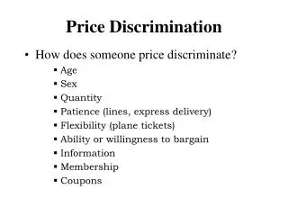
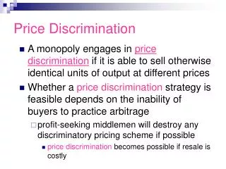
What is price discrimination? Price discrimination is the practice of selling the same product to different buyers (or groups of buyers) at different prices.
Examples of price discrimination • Airlines charge full fares to business travelers, whereas they offer discount fares to vacationers. • “Sizing up their income” pricing by dentists, plumbers, and auto mechanics. • Publishers of academic journals charge higher prices for library as compared to individual subscriptions. • Senior citizen discounts. • Discounts for new buyers—e.g., magazine subscriptions. • Theater ticket pricing
When is price discrimination feasible? • The seller must be capable of identifying market segments that differ based on willingness to pay, or elasticity of demand. • The seller must be capable of “enforcing” the different prices charged to different market segments—that is, the seller must be able to prevent “arbitrage.”
1st degree price discrimination • Sometimes called “perfect” price discrimination, the seller charges each buyer their “reservation price” for every unit purchased. • Reservation price is the maximum price a buyer is willing to pay rather than go without the last unit of the good.
Auctions Auctions are designed to force buyers nearer to their reservations prices.
The Cigarette Czar • Suppose an individual gained monopoly control of the supply of cigarettes in a particular geographic location. • The cigarette czar could practice 1st degree price discrimination by holding out until smokers paid their reservation price for each smoke.
3rd degree price discrimination This is the practice of charging different prices in different market segments
Examples of market “segments” • Business travelers versus tourists. • Kids versus adults • Those covered by health insurance and those not covered. • Senior citizens versus everyone else. • Mercedes Benz owners versus Chevrolet owners. • Domestic versus foreign buyers
Multinational pricing of autos The problem for a car manufacturer is to establish profit-maximizing prices on cars sold domestically and in the foreign market segment
The Demand Functions The inverse demand equation for the home (H) market is given by: Where PH is the price charge in the home market and H is the quantity sold in the home market The inverse demand equation for the foreign (F) market is given by:
The demand for cars 30,000 Foreign 25,000 Price Home 0 35.7 60 Quantity
Profit maximization in the Home segment 30,000 To maximize profits in the Home segment, set MRH = MCH 20,000 Price 10,000 MCH DH MRH 0 20 30 60 Quantity (000s)
Profit-maximization in the foreign market segment 25,000 To maximize profits in the Foreign segment, set MRF = MCF Price 18,000 MCF 11,000 MRF DF 0 10 35.7 60 Quantity (000s)
Summary Notice that the price is higher in the Home market where the manufacturer faces a less elastic demand curve
Interdependent demand Consider a microbrewery that brews lager and pilsner. The price of the lager will likely affect the demand for pilsner.
Example Let A denote lager and B is pilsner. Let the profit function be given by: Note: We assume that there are no interdependencies or complementarities in production
Determining the optimal quantity Produce up to the point in which the extra total revenue (MTR) from the sale of product A is equal to the marginal cost of A, and similarly for B. That is: And:
Numerical example Let MCA = $80; MCB = $40 PA = 280 – 2QA PB = 180 – QB – 2QA Notice that increased sales of A adversely affect sales of B, but not vice versa.
Thus we have: TR = RA + RB = (280QA – 2QA2) + (180QB – QB2-2QAQB) Therefore: MTRA= 280 – 4QA – 2QB And: MTRB= 180 – 2QB – 2QA So set MTRA = MCA and MTRB =MCB and solve for QA and QB The result is a linear equation system with two equations and two unknowns 280 – 4QA – 2QB = 80180 – 2QB – 2QA = 40
The solutions Solving the equation system yields: QA = 30 and QB = 40 Substituting into the price (or inverse demand) equations yields: PA = $220 and PB = $80 Contrast this outcome to the case where the brewery ignored the cross effect of A and B and simply tried to maximize profits from A.