Fluid Surface Rendering in CUDA
310 likes | 453 Views
Fluid Surface Rendering in CUDA. Andrei Monteiro Marcelo Gattass Assignment 4 June 2010. Topics. Introduction Related Work Algorithm CUDA Implementation Shading Results Conclusion References. Introduction. Fluids are part of our daily lives. Difficult to reproduce

Fluid Surface Rendering in CUDA
E N D
Presentation Transcript
Fluid Surface Rendering in CUDA Andrei Monteiro Marcelo Gattass Assignment 4 June 2010
Topics • Introduction • Related Work • Algorithm • CUDA Implementation • Shading • Results • Conclusion • References
Introduction • Fluids are part of our daily lives. • Difficult to reproduce • Simulations are expensive • Water • Smoke • Explosions • It is typically simulated off-line and then visualized. • In this work we are focusing in rendering the fluid in real time.
Introduction • Fluids are simulated using particle system using the Smoothed-Particle Hydrodynamics (SPH) method • It is made up of thousands to millions of particles (in a large scale simulation) • The objective is to extract the isosurface from this cluster of particles.
Introduction 262,144 particles
Introduction • Surface Rendering techniques • Marching Cubes • Point Splatting • Surfels • In this work, we use the Marching Cubes tecnique which is faster than the others.
Related Work • NVIDIA´s Notes on Parallel Marching Cubes Algorithm • Screen Space Fluid Rendering with Curvature Flow, Simon Green , NVIDIA • LORENSEN, W. E., AND CLINE, H. E. 1987. Marching cubes: A high resolution 3d surface construction algorithm. SIGGRAPH, Comput. Graph. 21, 4, 163–169. • Real-Time Animation of Water, Takashi Amada.
Algorithm • Marching Cubes • Is based on a grid method where it evaluates a scalar field on the vertices. • We take advantage of the Uniform Grid already implemented in our SPH simulation. • If the scalar field on a vertex is less than a threshold (isosurface value), the vertex is inside the isosurface / fluid and outside otherwise. • The most difficult part of the algorithm is to obtain a good scalar field function as the smoothness of the surface generated depends greatly on it. • We then use these information to triangulate the surface. • Normals are also calculated using, for example, the gradient of the scalar field.
Algorithm outside isosurface inside
Algorithm outside inside
Algorithm • Same algorithm applies in 3D, but the there are 256 voxel-triangle configurations: • 8 vertices per voxel • Total number of configurations is 28 = 256. • However, if we rotate and/or reflect the 15 cases below, we obtain 256 configurations. • In this work we use all 256 configurations.
CUDA Implementation • Triangle configurations (number of vertices, triangles) are stores in tables and written in textures. • Calculate number of vertices needed per voxel. • Count number of occupied voxels (excluding empy voxels with which do not contain the isosurface). • Compact the occupied voxels to be tightly packed. • Count the total number of vertices used to generate the surface. • Generate the triangles.
CUDA Implementation 1. Calculate number of vertices needed per voxel. • 1 thread per voxel • Check if 8 corners have scalar fields less than the isosurafce value. • If so, increment voxel vertex counter. • Use the vertex counter to access the Vertices Table, which contains the number of vertices with that specific configuration.
CUDA Implementation 2. Count number of occupied voxels • The previous step returns an array with the number of vertices per voxel and an array indicating if each voxel is occupied (1) or not (0). • Scan this array and return the number of occupied voxels. • Array elements with 0 indicates an unoccupied voxel. • Use the cudppScan from SDK, a fast scan function.
CUDA Implementation 3. Compact the occupied voxels to be tightly packed • The previous step returns an array of occupied scan where elements = 1 (occupied) have their values changed to the occupied index (0,1,2,3...), and elements = 0 have their values unchanged. • This kernel compacts the occupied voxels indices by looking at the occupied scan array values. 1 0 1 1 0 0 1 1 1 Occupied Array 0 0 1 2 0 0 3 4 5 Scanned Occupied Array 0 2 3 6 7 8 0 0 0 Compacted Voxel Array int index= current Thread; if (voxelOccupied[index] ) { compactedVoxelArray[ voxelOccupiedScan[index] ] = index; }
CUDA Implementation 4. Count the total number of vertices used to generate the surface. • Same idea of step 2. Use cudppScan to accumulate the number of vertices in each voxel position in the array.
CUDA Implementation 5. Generate Triangles • Use all information obtained in the previous steps. • 1 thread per occupied voxel. • Each thread obtains the current voxel index from the compacted voxel Array and use it to access the data such as number of vertices and scalar fields. • Linearly interpolate vertices and normals from each voxel edge:
CUDA Implementation f0 f0 f0 f1 f1 f1 f0 = scalar field´s value and gradient from one edge vertex; f1 = scalar field´s value and gradient from other edge vertex; float t = (isolevel - f0.w) / (f1.w - f0.w); p = lerp(p0, p1, t); n.x = lerp(f0.x, f1.x, t); n.y = lerp(f0.y, f1.y, t); n.z = lerp(f0.z, f1.z, t);
CUDA Implementation • Scalar Field: • Use density as scalar field • Normals are obtained by: ρs Density in a position r Kernel function ρi,j+1 Grid ρi,j ρi+1,j ρi-1,j ρi,j-1
Shading • Use Fresnel • Environment Mapping • Use Cube Texture • Reflection • Cube Mapping texture acces • Refraction • Cube Mapping texture access a = refracted color b = reflected scene color T = thickness function
Conclusion • The user was able to render a fluid with physical effects. • CUDA marching cubes proved to be fast. • Difficulty in obtaining a scalar field. • Can calculate normals per vertex.
References • NVIDIA´s Notes on Parallel Marching Cubes Algorithm. • Screen Space Fluid Rendering with Curvature Flow, Simon Green , NVIDIA. Retrieved Jun 25, 2010. • LORENSEN, W. E., AND CLINE, H. E. 1987. Marching cubes: A high resolution 3d surface construction algorithm. SIGGRAPH, Comput. Graph. 21, 4, 163–169. • Real-Time Animation of Water, Takashi Amada. • NVIDIACUDA Programming Guide. V. 2.0, 2008. Retrieved Mar 29, 2010.