Download

1 / 50
500 likes | 647 Views
This document provides an in-depth exploration of advanced algorithms for data compression, focusing on Huffman codes and prefix codes. It highlights the significance of Huffman's algorithm, which generates optimal prefix codes used in various compression applications like gzip and jpeg. The text explains the properties of Huffman coding, running examples, and the concept of entropy as a measure of information. It also addresses the performance, optimality, and practical implementation of Huffman codes, including encoding and decoding processes, alongside challenges faced in specific scenarios. ###

E N D
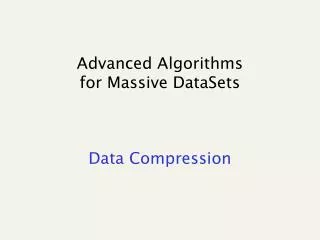
Advanced Algorithms for Massive DataSets Data Compression
0 1 a 0 1 d b c Prefix Codes A prefix code is a variable length code in which no codeword is a prefix of another one e.g a = 0, b = 100, c = 101, d = 11 Can be viewed as a binary trie 0 1
Huffman Codes Invented by Huffman as a class assignment in ‘50. Used in most compression algorithms • gzip, bzip, jpeg (as option), fax compression,… Properties: • Generates optimalprefix codes • Fast to encode and decode
0 1 1 (.3) 1 0 (.5) 0 (1) Running Example p(a) = .1, p(b) = .2, p(c ) = .2, p(d) = .5 a(.1) b(.2) c(.2) d(.5) a=000, b=001, c=01, d=1 There are 2n-1 “equivalent” Huffman trees
Entropy (Shannon, 1948) For a source S emitting symbols with probability p(s), the self information of s is: bits Lower probability higher information Entropy is the weighted average of i(s) i(s) 0-th order empirical entropy of string T
Performance: Compression ratio Compression ratio = #bits in output / #bits in input Compression performance: We relate entropy against compression ratio. Empirical H vs Compression ratio Shannon In practice Avgcw length p(A) = .7, p(B) = p(C) = p(D) = .1 H≈ 1.36 bits Huffman ≈ 1.5 bits per symb
Problem with Huffman Coding • We can prove that (n=|T|): n H(T) ≤ |Huff(T)| < n H(T) + n which looses < 1 bit per symbol on avg!! • This loss is good/bad depending on H(T) • Take a two symbol alphabet = {a,b}. • Whichever is their probability, Huffman uses 1 bit for each symbol and thus takes n bits to encode T • If p(a) = .999, self-information is: bits << 1
Data Compression Huffman coding
Huffman Codes Invented by Huffman as a class assignment in ‘50. Used in most compression algorithms • gzip, bzip, jpeg (as option), fax compression,… Properties: • Generates optimal prefix codes • Cheap to encode and decode • La(Huff) = H if probabilities are powers of 2 • Otherwise, La(Huff)< H +1 < +1 bit per symb on avg!!
0 1 1 (.3) 1 0 (.5) 0 (1) Running Example p(a) = .1, p(b) = .2, p(c ) = .2, p(d) = .5 a(.1) b(.2) c(.2) d(.5) a=000, b=001, c=01, d=1 There are 2n-1 “equivalent” Huffman trees What about ties (and thus, tree depth) ?
Encoding and Decoding Encoding: Emit the root-to-leaf path leading to the symbol to be encoded. Decoding: Start at root and take branch for each bit received. When at leaf, output its symbol and return to root. 1 0 (.5) d(.5) abc... 00000101 1 0 (.3) 101001... dcb c(.2) 0 1 a(.1) b(.2)
Huffman’s optimality Averagelength of a code = Averagedepth of itsbinary trie • Reducedtree= tree on (k-1) symbols • substitutesymbols x,z with the special “x+z” RedT T d d +1 +1 “x+z” x z LRedT= ….+ d *(px+ pz) LT = ….+ (d+1)*px+ (d+1)*pz LT = LRedT+ (px+ pz)
Huffman’s optimality ClearlyHuffmanisoptimalfor k=1,2 symbols By induction: assume that Huffman is optimal for k-1 symbols, hence LRedH(p1, …, pk-2, pk-1 + pk) is minimum Now, take k symbols, where p1 p2 p3 … pk-1 pk ClearlyLopt(p1, …, pk-1 , pk) = LRedOpt(p1, …, pk-2, pk-1 + pk) + (pk-1 + pk) optimal on k-1 symbols (byinduction), herethey are (p1, …, pk-2, pk-1 + pk) LOpt= LRedOpt[p1, …, pk-2, pk-1 + pk]+ (pk-1 + pk) LRedH[p1, …, pk-2, pk-1 + pk]+ (pk-1 + pk) = LH
Model size may be large Huffman codes can be made succinct in the representation of the codeword tree, and fast in (de)coding. Canonical Huffman tree We store for any level L: • firstcode[L] • Symbols[L], for each level L = 00.....0
Canonical Huffman (.4) (.6) (.1) (.04) (.02) (.02) 1(.3) 2(.01) 3(.01) 4(.06) 5(.3) 6(.01) 7(.01) 1(.3) 2 5 5 3 2 5 5 2
CanonicalHuffman: Main idea.. SymbLevel 1 2 2 5 3 5 4 3 5 2 6 5 7 5 8 2 Wewant a treewiththisform WHY ?? 1 5 8 4 2 3 6 7 It can be stored succinctly using two arrays: • firstcode[]= [--,01,001,00000] = [--,1,1,0] (as values) • Symbols[][]= [ [], [1,5,8], [4], [], [2,3,6,7] ]
CanonicalHuffman: Main idea.. SymbLevel 1 2 2 5 3 5 4 3 5 2 6 5 7 5 8 2 1 5 8 4 sort 2 3 6 7 numElem[] = [0, 3, 1, 0, 4] Symbols[][]= [ [], [1,5,8], [4], [], [2,3,6,7] ] Firstcode[5] = 0 Firstcode[4] = ( Firstcode[5] + numElem[5] ) / 2 = (0+4)/2 = 2 (= 0010 since it is on 4 bits)
CanonicalHuffman: Main idea.. SymbLevel 1 2 2 5 3 5 4 3 5 2 6 5 7 5 8 2 Value 2 Value 2 1 5 8 4 sort 2 3 6 7 numElem[] = [0, 3, 1, 0, 4] Symbols[][]= [ [], [1,5,8], [4], [], [2,3,6,7] ] • firstcode[]= [2, 1, 1, 2, 0] T=...00010...
CanonicalHuffman: Decoding Value 2 Value 2 1 5 8 Succint and fast in decoding Firstcode[]= [2, 1, 1, 2, 0] Symbols[][]= [ [], [1,5,8], [4], [], [2,3,6,7] ] 4 2 3 6 7 T=...00010... Decoding procedure Symbols[5][2-0]=6
Problem with Huffman Coding Take a two symbol alphabet = {a,b}. Whichever is their probability, Huffman uses 1 bit for each symbol and thus takes n bits to encode a message of n symbols This is ok when the probabilities are almost the same, but what about p(a) = .999. The optimal code for a is bits So optimal coding should use n *.0014 bits, which is much less than the n bits taken by Huffman
What can we do? Macro-symbol = block of k symbols • 1 extra bit per macro-symbol = 1/k extra-bits per symbol • Larger model to be transmitted: |S|k(k * log |S|) + h2 bits (where h might be |S|) Shannon took infinite sequences, and k ∞ !!
Data Compression Dictionary-based compressors
LZ77 Algorithm’s step: • Output <dist, len, next-char> • Advance by len + 1 A buffer “window” has fixed length and moves a a c a a c a b c a a a a a a a c <6,3,a> Dictionary(all substrings starting here) a c a a c a a c a b c a a a a a a c <3,4,c>
LZ77 Decoding Decoder keeps same dictionary window as encoder. • Finds substring and inserts a copy of it What if l > d? (overlap with text to be compressed) • E.g. seen = abcd, next codeword is (2,9,e) • Simply copy starting at the cursor for (i = 0; i < len; i++) out[cursor+i] = out[cursor-d+i] • Output is correct: abcdcdcdcdcdce
LZ77 Optimizations used by gzip LZSS: Output one of the following formats (0, position, length)or(1,char) Typically uses the second format if length < 3. Special greedy: possibly use shorter match so that next match is better Hash Table for speed-up searches on triplets Triples are coded with Huffman’s code
LZ-parsing (gzip) 0 # s i 1 12 si p 1 i 3 ssi mississippi# 2 ppi# 1 ppi# ssippi# 4 ppi# # ssippi# 6 3 i# ppi# pi# ssippi# 7 4 11 8 5 2 1 10 9 <m><i><s><si><ssip><pi> T = mississippi# 1 2 4 6 8 10
LZ-parsing (gzip) It is on the path to 6 0 # s By maximality check only nodes i 1 12 p 1 Leftmost occ = 3 < 6 si i 3 ssi mississippi# 2 ppi# 1 ppi# ssippi# 4 Leftmost occ = 3 < 6 ppi# # ssippi# 6 3 i# ppi# pi# ssippi# 7 4 11 8 5 2 1 10 9 <ssip> Longest repeated prefix of T[6,...] Repeat is on the left of 6 T = mississippi# 1 2 4 6 8 10
LZ-parsing (gzip) min-leaf Leftmost copy 0 # s 3 i 1 12 si 2 p 1 Parsing: Scan T Visit ST and stop when min-leaf ≥ current pos 3 i 3 ssi 4 mississippi# 9 2 2 ppi# 1 ppi# ssippi# 4 ppi# # ssippi# 6 3 i# ppi# pi# ssippi# 7 4 11 8 5 2 1 10 9 <m><i><s><si><ssip><pi> Precompute the min descending leaf at every node in O(n) time. T = mississippi# 1 2 4 6 8 10
Possiblybetterfor cache effects LZ78 Dictionary: • substrings stored in a trie (each has an id). Coding loop: • find the longest match S in the dictionary • Output its id and the next character c after the match in the input string • Add the substring Scto the dictionary Decoding: • builds the same dictionary and looks at ids
LZ78: Coding Example Output Dict. 1 = a (0,a) a a b a a c a b c a b c b 2 = ab (1,b) a a b a a c a b c a b c b 3 = aa (1,a) a a b a a c a b c a b c b 4 = c (0,c) a a b a a c a b c a b c b 5 = abc (2,c) a a b a a c a b c a b c b 6 = abcb (5,b) a a b a a c a b c a b c b
a 2 = ab (1,b) a a b 3 = aa (1,a) a a b a a 4 = c (0,c) a a b a a c 5 = abc (2,c) a a b a a c a b c 6 = abcb (5,b) a a b a a c a b c a b c b LZ78: Decoding Example Dict. Input 1 = a (0,a)
Lempel-Ziv Algorithms Keep a “dictionary” of recently-seen strings. The differences are: • How the dictionary is stored • How it is extended • How it is indexed • How elements are removed • How phrases are encoded LZ-algos are asymptotically optimal, i.e. their compression ratio goes to H(T) for n !! No explicit frequency estimation
Web Algorithmics File Synchronization
File synch: The problem client wants to update an out-dated file server has new file but does not know the old file update without sending entire f_new(using similarity) rsync: file synch tool, distributed with Linux request f_new f_old update Server Client
The rsync algorithm hashes f_new f_old encoded file Server Client
The rsync algorithm (contd) • simple, widely used, single roundtrip • optimizations: 4-byte rolling hash + 2-byte MD5, gzipfor literals • choice of block size problematic (default: max{700, √n} bytes) • not good in theory: granularity of changes may disrupt use of blocks Gzip
Simple compressors: too simple? • Move-to-Front (MTF): • As a freq-sortingapproximator • As a caching strategy • As a compressor • Run-Length-Encoding (RLE): • FAX compression
Move to Front Coding Transforms a char sequence into an integersequence, that can then be var-length coded • Start with the list of symbols L=[a,b,c,d,…] • For each input symbol s • output the position of s in L • move s to the front of L Properties: • Exploit temporal locality, and it is dynamic • X = 1n 2n 3n… nn Huff = O(n2 log n), MTF = O(n log n) + n2 There is a memory
Run Length Encoding (RLE) If spatial locality is very high, then abbbaacccca => (a,1),(b,3),(a,2),(c,4),(a,1) In case of binary strings just numbers and one bit Properties: • Exploit spatial locality, and it is a dynamic code • X = 1n 2n 3n… nn Huff(X) = O(n2 log n) >Rle(X) = O( n (1+log n) ) There is a memory
Data Compression Burrows-Wheeler Transform
# mississipp i i #mississipp i ppi#mississ i ssippi#miss i ssissippi# m Sort the rows m ississippi# T p i#mississi p p pi#mississ i s ippi#missi s s issippi#mi s s sippi#miss i s sissippi#m i The Burrows-Wheeler Transform (1994) Let us given a text T = mississippi# F L mississippi# ississippi#m ssissippi#mi sissippi#mis issippi#miss ssippi#missi sippi#missis ippi#mississ ppi#mississi pi#mississip i#mississipp #mississippi
A famous example Much longer...
L is highly compressible Algorithm Bzip : • Move-to-Front coding of L • Run-Length coding • Statistical coder Compressing L seems promising... Key observation: • L is locally homogeneous • Bzip vs. Gzip: 20% vs. 33%, but it is slower in (de)compression !
SA L BWT matrix 12 11 8 5 2 1 10 9 7 4 6 3 #mississipp i#mississip ippi#missis issippi#mis ississippi# mississippi pi#mississi ppi#mississ sippi#missi sissippi#mi ssippi#miss ssissippi#m i p s s m # p i s s i i Given SA and T, we have L[i] = T[SA[i]-1] How to compute the BWT ? We said that: L[i] precedes F[i] in T #mississipp i#mississip ippi#missis issippi#mis ississippi# mississippi pi#mississi ppi#mississ sippi#missi sissippi#mi ssippi#miss ssissippi#m L[3] = T[ 7 ]
i ssippi#miss How do we map L’s onto F’s chars ? i ssissippi# m ... Need to distinguishequal chars in F... m ississippi# p i#mississi p p pi#mississ i s ippi#missi s s issippi#mi s s sippi#miss i s sissippi#m i Take two equal L’s chars Rotate rightward their rows Same relative order !! A useful tool: L F mapping F L unknown # mississipp i i #mississipp i ppi#mississ
Two key properties: 1. LF-array maps L’s to F’s chars 2. L[ i ] precedes F[ i ] in T i ssippi#miss i ssissippi# m m ississippi# p p i T = .... # i p i#mississi p p pi#mississ i s ippi#missi s s issippi#mi s s sippi#miss i s sissippi#m i InvertBWT(L) Compute LF[0,n-1]; r = 0; i = n; while (i>0) { T[i] = L[r]; r = LF[r]; i--; } The BWT is invertible F L unknown # mississipp i i #mississipp i ppi#mississ Reconstruct T backward:
# at 16 Mtf = [i,m,p,s] Alphabet |S|+1 An encoding example T = mississippimississippimississippi L = ipppssssssmmmii#pppiiissssssiiiiii Mtf = 020030000030030 300100300000100000 Mtf = 030040000040040 400200400000200000 Bin(6)=110, Wheeler’s code RLE0 = 03141041403141410210 Bzip2-output = Huffman on |S|+1 symbols... ... plus g(16), plus the original Mtf-list (i,m,p,s)