Download

1 / 42
430 likes | 508 Views
Understand transforming curved lines into straight ones, homogeneity of error variance, estimating mean & standard deviation. Learn Probit Analysis through examples and optimizing yield-nitrogen applications. Exploring yield-nitrogen intersections and bivariate distribution correlation.

E N D
Making a curved line straight Data Transformation & Regression
Last Class • Predicting the dependant variable and standard errors of predicted values. • Outliers. • Need to visually inspect data in graphic form. • Making a curved line straight. • Transformation.
Early Growth Pattern of Plants y = Ln(y)
Homogeneity of Error Variance y =Ln(y)
Growth Curve Y = ex
Growth Curve Y = Log(x)
Sigmoid Growth Curve Accululative Normal Distribution
Sigmoid Growth Curve ƒ(dd T - Accululative Normal Distribution T
Sigmoid Growth Curve ƒ(dd T - Accululative Normal Distribution T
Probit Analysis • Group of plants/insects exposed to different concentrations of a specific stimulant (i.e. insecticide). • Data are counts (or proportions), say number killed. • Usually concerned or interested in concentration which causes specific event (i.e. LD 50%).
Estimating the Mean y= 50% Killed x ~ 2.8
Estimating the Standard Deviation 95% values 2 2.8
Estimating the Standard Deviation = 1.2 95% values 2 2.8
Probit Analysis Probit () = + . Log10(concentration) = -1.022 + 0.202 = 2.415 + 0.331 Log10 (conc) to kill 50% (LD-50) is probit 0.5 = 0 0 = -1.022 + 2.415 x LD-50 LD-50 = 0.423 100.423 = 2.65%
Problems • Obtaining “good estimates” of the mean and standard deviation of the data. • Make a calculated guess, use iteration to get “better fit” to observed data.
Optimal Assent Y1=a1+b1x
Optimal Assent Y2=a2+b2x Y1=a1+b1x
Optimal Assent t =[b1-b2]/se(b) = ns Y2=a2+b2x Y1=a1+b1x
Optimal Assent Y3=a3+b3x Y1=a1+b1x
Optimal Assent Y3=a3+b3x t =[b1-b3]/se(b) = *** Y1=a1+b1x
Optimal Assent Y3=a3+b3x Y1=a1+b1x
Optimal Assent t =[b1-bn]/se(b) = *** Yn=an+bnx Y3=a3+b3x Y1=a1+b1x
Optimal Assent Y3=a3+b3x Y3=a3+b3x Y1=a1+b1x
What application of nitrogen will result in the optimumyield response?
Intersecting Lines Y = 9.01x + 466.60 Y = 2.81x + 1055.10
Intersecting Lines t = [b11 - b21]/average se(b) 6.2/0.593 = 10.45 * , With 3 df Intersect = same value of y b10 + b11x = y = b20 + b21x x = [b20 - b10]/[b11 - b21] = 94.92 lb N/acre with 1321.83 lb/acre seed yield
Intersecting Lines Y = 9.01x + 466.60 1321.83 lb/acre Y = 2.81x + 1055.10 94.92 lb N/acre
Linear Y = b0 + b1x Quadratic Y = b0 + b1x + b2 x2 Cubic Y = b0 + b1x + b2 x2 + b3 x3 Bi-variate Distribution Correlation