Optically polarized atoms
210 likes | 341 Views
This chapter delves into the intricate dynamics of coherence and excitation in atomic systems when subjected to optically polarized light. It explores exciting 0-to-1 transitions with both z and x polarized light, emphasizing the coherent superposition of states and the significance of excitation rates between different levels, such as J'' = 0. Key phenomena such as Electromagnetically Induced Transparency (EIT), Coherent Population Trapping (CPT), and Quantum Beats are discussed. The implications of these effects, including their relevance in quantum optics and laser physics, are analyzed, providing insight into advanced methods for controlling atomic states.

Optically polarized atoms
E N D
Presentation Transcript
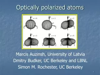
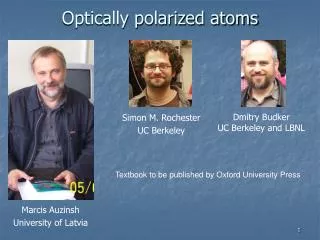
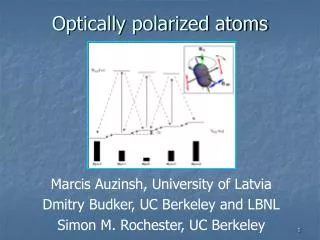
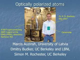
Optically polarized atoms Marcis Auzinsh, University of Latvia Dmitry Budker, UC Berkeley and LBNL Simon M. Rochester, UC Berkeley
Chapter 6: Coherence in atomic systems • Exciting a 01 transition with z polarized light • Things are straightforward: the |1,0> state is excited • What if light is x polarized ?
Exciting a 01 transition with x polarized light • x • Note: light is in a superposition of σ+and σ - Recipe for finding how much of a given basic polarization is contained in the field E
Exciting a 01 transition with x polarized light • Coherent superposition -|1,-1>+|1,1> is excited • Why do we care that a coherent superposition is excited? • Suppose we want to further excite atoms to a level J’’
Compare excitation rate to J’’=0 for x and y polarized E ’ light
Compare excitation rate to J’’=0 for x and y polarized E ’ light • Calculate final-state amplitude as • with • First, for x polarized light Now repeat for y polarized light !
Compare excitation rate to J’’=0 for x and y polarized E ’ light • For y polarized light : • Or, with a common phase factor • So, finally, we have :
y polarized light x polarized light
The state we prepared with x polarized light E is a bright state for x polarized light E ’ • At the same time, it is a dark statefor y polarized light E ’ • A quantum interference effect ! • Two pathways from the initial to final state; constructive or destructive interference • This is the basic phenomenon underlying : • EIT electromagnetically induced transparency • CPT coherent population trapping • STIRAP stimulated Raman adiabatic passage • NMOR nonlinear magneto-optical rotation • LWI lasing w/o inversion • “slow light” very slow and superluminal group velocities • coherent control of chemical reactions • …
An important comment about bases • We have considered excitation with x polarized Elight, and have seen an “interesting” coherence effect (darkand bright) excited states • If we choose quantization axis along light polarization, things look trivial Bright intermediate state for z polarized light E’ Darkintermediate state for x or y polarized light E’
Quantum Beats • Suppose we prepare a coherent superposition of energy eigenstates with different energies • For example, we can be exciting Zeeman sublevels that are split by a magnetic field • The wavefunction will be something like
Quantum Beats • As a specific example, again consider exciting a 01 transition with x polarized light • Assume short, broadband excitationpulse at t=0. Then, at a later time:
Quantum Beats • Now, as before, we excite further with second cw (but spectrally broad and weak) light field • The amplitude of excitation depends on time:
Quantum Beats • Excitation probability is harmonically modulated • Modulation frequency energy intervals between coherently excited states • The evolution of the intermediate state can be seen on the plots of electron density • Note: Electron density plots are NOT the same as the angular-momentum probability plots we use a lot in this course !
Quantum Beats • In this case temporal evolution is simple – it is just Larmor precession
Quantum Beats • Q: What will be seen with y polarized light E ’ ? • A: The same but with opposite phase x: y: • Quantum beats in atomic spectroscopy were discovered in 1960s by E. B. Alexandrov in USSR and J.N. Dodd, G.W.Series, and co-workers in UK
The Hanle Effect • Now introduce relaxation: assume that amplitude of state J’ decays at rate Γ/2 • Amplitudes of excited sublevels evolve according to : • With x polarized second excitation E’ , we have
The Hanle Effect • Assuming that both light fields are cw, and that we are detecting steady-state signals as a function of magnetic field, we have: • Limiting cases: • This is a nice method for determining lifetimes that does not require fast excitation, photodetectors, or electronics
The Hanle Effect • What’s going on is clearly seen on electron-density plot for J’
The Hanle Effect • A similar illustration can be done with angular-momentum probability plots • Quite similar physics takes place in Nonlinear Faraday Effect • Transverse (w.r.t. magnetic field) alignment converted to longitudinal alignment • The Hanle effect is sometimes called magnetic depolarization of radiation. This refers to observation via emission from the polarized state