NATS 101 Section 13: Lecture 24
290 likes | 467 Views
NATS 101 Section 13: Lecture 24. Weather Forecasting Part I. Forecasting weather and climate is REALLY important—and that is the main reason why use our tax dollars to do it!. Goes to the core of one of reasons to study weather and climate I mentioned the first day of class.

NATS 101 Section 13: Lecture 24
E N D
Presentation Transcript
NATS 101 Section 13: Lecture 24 Weather Forecasting Part I
Forecasting weather and climate is REALLY important—and that is the main reason why use our tax dollars to do it! Goes to the core of one of reasons to study weather and climate I mentioned the first day of class.
So how can we solve the problem? Simple approach vs. complex approach The simple forecasting approaches should be used as a “sanity check” to see if the complex approach are worth it.
Simple Approach #1Persistence Forecast Persistence: Future atmospheric state is the same as the current state. Good Example: Tropical rainforest during wet season. It’s raining today, so predict rain for tomorrow. How is this related to the general circulation? TODAY THURSDAY FRIDAY HIGH: 83°F LOW: 70°F HIGH: 83°F LOW: 70°F HIGH: 83°F LOW: 70°F
Simple Approach #2Trend forecast Trend: Add past change to current condition to obtain forecast for future state Good Example: Temperature in Tucson increasing at 3°F per hour in the morning on a clear, calm day. Use this to forecast temperatures later in afternoon because the surface heats at a steady rate due to solar heating. 9 AM 12 PM 3 PM 96°F 99°F 93°F
Simple Approach #3Climatology forecast Climatology: Forecast future state as the average of past weather for a given period Good example: Forecast about six inches of rain to occur during the monsoon in Tucson, the average for the 1971-2000 period.
Simple approach #4: Analog forecast Analog: Find a previous atmospheric state that is like the current state and forecast the same evolution. This one does require some more skill because no two situations are EVER exactly alike… Good example: If a surface low pressure forms in the eastern Gulf of Mexico with a deep upper-level trough to the west, a Nor’ester will roll up the Eastern seaboard—like the 1993 Superstorm 500-mb MAP: 1993 Superstorm SURFACE MAP: 1993 Superstorm LOW TRACK
The complicated way to make a forecast is to use a physical and mathematical model of the atmosphere, starting from an observed state at an initial time. This is called Numerical Weather Prediction (NWP)
Why do Numerical Weather Prediction? NUMERICAL WEATHER PREDICTION IS ONLY USEFUL IF YOU CAN SHOW IT DOES WHAT?
Steps in Numerical Weather Prediction • ANALYSIS: Gather the data (from various sources) • PREDICTION: Run the NWP model • POST-PROCESSING: Display and use products
Analysis Phase: Surface data Surface data comes from surface meteorological stations and ships at sea.
ASOS: Automated Surface Observing System Electronic sensors to measure all elements of weather: Temperature Pressure Moisture Wind speed and direction Visibility Precipitation and precipitation type Located at virtually every major airport. Many observations you see on a surface map are taken from ASOS.
Analysis phase: Ocean data Drifting and moored ocean buoys. TAO ARRAY TAO ARRAY
Analysis Phase:Upper air data from radiosondes (weather balloons)
Geostationary Polar Orbit Analysis Phase: Satellites Geostationary: Fixed over one location at all times directly over equator. Polar: Orbit over the poles, covering the Earth in swaths.
So we get all that data, say about every six hours or so. Now what?
Objective Analysis Data must be interpolated to some kind of grid so we can run the numerical weather prediction model—this is called the initial analysis. For a regional model these are equally spaced points. Grid spacing = 35 km
Now the “fun” begins—actually running the model to make a prediction! But how do NWP models work? Not a simple answer!!
Structure of atmospheric models Dynamical Core Mathematical expressions of Conservation of motion (i.e. Newton’s 2nd law F = ma) Conservation of mass Conservation of energy Conservation of water These must be discretized to solve on a grid at given time interval, starting from the initial conditions (analysis). Parameterizations One dimensional column models which represent processes that cannot be resolved on the grid. Called the model “physics”—but it is essentially engineering code.
Equations represented in dynamic coreMUST SOLVE AT EVERY GRID POINT! MASS CONSERVATION ENERGY CONSERVATION CONSERVATION OF MOTION CONSERVATION OF MOISTURE (Pielke 2002) Why is just doing this REALLY, REALLY HARD? Have to __________ the equations, so they can be solved on a grid. Are the equations linear or non-linear? We haven’t even accounted for parameterizations yet!
Parameterized processesOne-dimensional models MOST OF THESE REPRESENTED AS 1-D PROCESSES—WITH ESSENTIALLY ENGINEERING CODE.
Turbulent diffusion Land surface energy balance Precipitation processes Radiation Dynamic core Discretized dynamical equations Boundary layer Boundary conditions
50 km “A Lot Happens Inside a Grid Box”(Tom Hamill, CDC/NOAA) Approximate Size of One Grid Box for NCEP Global Ensemble Model Note Variability in Elevation, Ground Cover, Land Use Rocky Mountains Denver Source: www.aaccessmaps.co
13 km Model Terrain Big mountain ranges, like the Sierra Nevada, are resolved. But isolated peaks, like the Catalina’s, are not evident. 100 m contour
Summary of Lecture 24 Weather and climate forecasting is really important, but a very challenging problem. Simple approaches to forecasting include: persistence, trend, climatology, and analog. It must be demonstrated that any other forecasting methodology can beat these to show it’s useful. NWP is the use of a physical and mathematical model to represent the atmosphere, starting from an observed state at an initial time. In the analysis phase of NWP, data is gathered from a variety of sources, such as: surface stations, buoys, radiosondes, aircraft, and satellites. These data are then objectively analyzed to a grid. A NWP model consists of a dynamical core and (one-dimensional) parameterizations to represent sub-grid scale processes. “Run” a NWP model by solving the dynamical equations and parameterizations forward in time.