Graphs II
450 likes | 570 Views
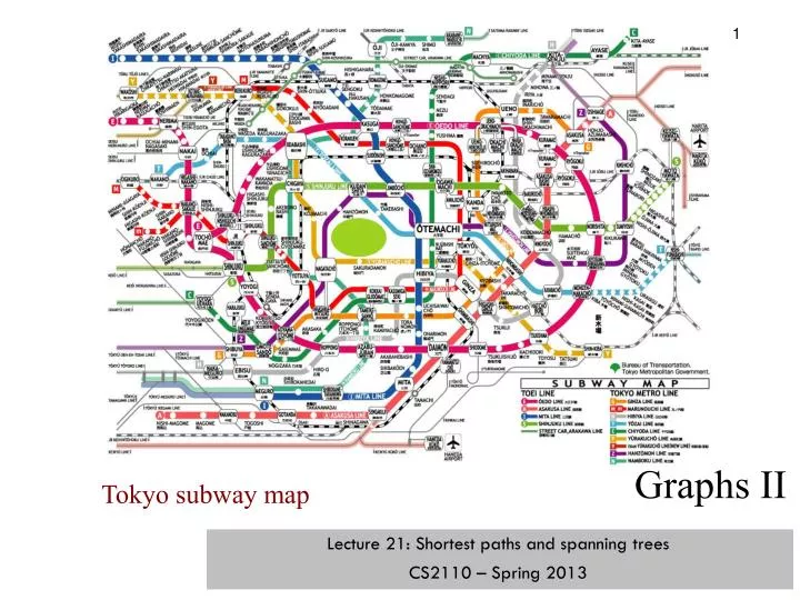
Graphs II. Lecture 21: Shortest paths and spanning trees CS2110 – Spring 2013. Tokyo subway map. "This 'telephone' has too many shortcomings to be seriously considered as a means of communications. ” Western Union, 1876

Graphs II
E N D
Presentation Transcript
Graphs II Lecture 21: Shortest paths and spanning trees CS2110 – Spring 2013 Tokyo subway map
"This 'telephone' has too many shortcomings to be seriously considered as a means of communications. ” Western Union, 1876 "I think there is a world market for maybe five computers.” Watson, chair of IBM, 1943 "The problem with television is that the people must sit and keep their eyes glued on a screen; the average American family hasn't time for it.” New York Times, 1949 "There is no reason anyone would want a computer in their home.” Ken Olson, founder DEC, 1977 "640K ought to be enough for anybody.” Bill Gates, 1981(Did he mean memory or money?) "By the turn of this century, we will live in a paperless society.” Roger Smith, chair GM, 1986 "I predict the Internet... will go spectacularly supernova and in 1996 catastrophically collapse.” Bob Metcalfe, 3Com founder, 1995
1 2 4 0 1 0 1 0 0 1 0 0 0 0 0 0 1 1 0 2 3 3 4 2 3 Representations of Graphs 1 2 4 3 Adjacency Matrix Adjacency List 1 2 3 4 1 2 3 4
Adjacency Matrix or Adjacency List? • Adjacency List • Uses space O(e+n) • Iterate over all edges in time O(e+n) • Answer “Is there an edge from u to v?” in O(d(u)) time • Better for sparse graphs (fewer edges) • Adjacency Matrix • — Uses space O(n2) • — Iterate over all edges edges in time O(n2) • — Answer “Is there an edge from u to v?” in O(1) time • — Better for dense graph (lots of edges) n: # vertices e: # edges d(u) = outdegree of u
Shortest paths in graphs 5 Problem of finding shortest (min-cost) path in a graph occurs often • Shortest route between Ithaca and New York City • Result depends on notion of cost: • Least mileage • Least time • Cheapest • Least boring • Can represent all these “costs” as edge weights How do we find a shortest path?
Dijkstra’s shortest-path algorithm 6 Edsger Dijkstra, in an interview in 2010 (Comm ACM53 (8): 41–47), said: … the algorithm for the shortest path, which I designed in about 20 minutes. One morning I was shopping in Amsterdam with my young fiance, and tired, we sat down on the cafe terrace to drink a cup of coffee, and I was just thinking about whether I could do this, and I then designed the algorithm for the shortest path. As I said, it was a 20-minute invention. [Took place in 1956] Dijkstra, E.W. A note on two problems in Connexion with graphs. Numerische Mathematik 1, 269–271 (1959). Visit http://www.dijkstrascry.com for all sorts of information on Dijkstra and his contributions. As a historical record, this is a gold mine.
Dijkstra’s shortest-path algorithm 7 Dijsktra describes the algorithm in English: • When he designed it in 1956, most people were programming in assembly language! • Only one high-level language: Fortran, developed by John Backus at IBM and not quite finished. No theory of order-of-execution time —topic yet to be developed. In paper, Dijsktra says, “my solution is preferred to another one … “the amount of work to be done seems considerably less.” Dijkstra, E.W. A note on two problems in Connexion with graphs. Numerische Mathematik 1, 269–271 (1959).
2 0 4 3 1 2 4 3 4 3 1 Dijkstra’s shortest path algorithm The n (> 0) nodes of a graph numbered 0..n-1. Each edge has a positive weight. weight(v1, v2) is the weight of the edge from node v1 to v2. Some node v be selected as the start node. Calculate length of shortest path from v to each node. Use an array L[0..n-1]: for each node w, store in L[w] the length of the shortest path from v to w. L[0] = 2 L[1] = 5 L[2] = 6 L[3] = 7 L[4] = 0 v
Dijkstra’s shortest path algorithm Develop algorithm, not just present it. Need to show you the state of affairs —the relation among all variables— just before each node i is given its final value L[i]. This relation among the variables is an invariant, because it is always true. Because each node i (except the first) is given its final value L[i] during an iteration of a loop, the invariant is called a loop invariant. L[0] = 2 L[1] = 5 L[2] = 6 L[3] = 7 L[4] = 0
Settled S f 2 0 Frontier F Far off f 4 3 1 2 4 3 4 3 1 The loop invariant (edges leaving the black set and edges from the blue to the red set are not shown) 1. For a Settled node s, L[s] is length of shortest v --> s path. 2.All edges leaving S go to F. 3.For a Frontier node f, L[f] is length of shortest v --> f path using only red nodes (except for f) 4.For a Far-off node b, L[b] = ∞ 5. L[v] = 0, L[w] > 0 for w ≠ v v
f g v f g Settled S Frontier F Far off Theorem about the invariant L[g] ≥ L[f] 1. For a Settled node s, L[s] is length of shortest v --> r path. 2.All edges leaving S go to F. 3.For a Frontier node f, L[f]is length of shortest v --> f path using only Settled nodes (except for f). 4.For a Far-off node b, L[b] = ∞. 5. L[v] = 0, L[w] > 0 for w ≠ v . Theorem. For a node f in F with minimum L value (over nodes in F), L[f] is the length of the shortest path from v to f. Case 1:v is in S. Case 2:v is in F. Note that L[v] is 0; it has minimum L value
The algorithm For all w, L[w]= ∞; L[v]= 0; S F Far off F= { v }; S= { }; v 1. For s, L[s] is length of shortest v-->s path. 2. Edges leaving S go to F. 3.For f, L[f]is length of shortest v --> f path using red nodes (except for f). 4.For b in Far off, L[b] = ∞ 5. L[v] = 0, L[w] > 0 for w ≠ v Loopy question 1: Theorem: For a node f in F with min L value, L[f] is shortest path length How does the loop start? What is done to truthify the invariant?
The algorithm For all w, L[w]= ∞; L[v]= 0; S F Far off F= { v }; S= { }; while { } F ≠ {} 1. For s, L[s] is length of shortest v-->s path. 2. Edges leaving S go to F. 3.For f, L[f]is length of shortest v --> f path using red nodes (except for f). 4.For b in Far off, L[b] = ∞ 5. L[v] = 0, L[w] > 0 for w ≠ v Loopy question 2: Theorem: For a node f in F with min L value, L[f] is shortest path length When does loop stop? When is array L completely calculated?
f f The algorithm For all w, L[w]= ∞; L[v]= 0; S F Far off F= { v }; S= { }; while { } F ≠ {} f= node in F with min L value;Remove f from F, add it to S; 1. For s, L[s] is length of shortest v-->s path. 2. Edges leaving S go to F. 3.For f, L[f]is length of shortest v --> f path using red nodes (except for f). 4.For b, L[b] = ∞ 5. L[v] = 0, L[w] > 0 for w ≠ v Loopy question 3: Theorem: For a node f in F with min L value, L[f] is shortest path length How is progress toward termination accomplished?
w w w The algorithm For all w, L[w]= ∞; L[v]= 0; S F Far off F= { v }; S= { }; while { } F ≠ {} f f= node in F with min L value;Remove f from F, add it to S; 1. For s, L[s] is length of shortest v-->s path. for each edge (f,w) { } if (L[w] is ∞) add w to F; 2. Edges leaving S go to F. 3.For f, L[f]is length of shortest v --> f path using red nodes (except for f). if (L[f] + weight (f,w) < L[w]) L[w]= L[f] + weight(f,w); 4.For b, L[b] = ∞ 5. L[v] = 0, L[w] > 0 for w ≠ v Algorithm is finished Loopy question 4: Theorem: For a node f in F with min L value, L[f] is shortest path length How is the invariant maintained?
if (L[w] == Integer.MAX_VAL) { L[w]= L[f] + weight(f,w); add w to F; } else L[w]= Math.min(L[w], L[f] + weight(f,w)); S F About implementation 1. No need to implement S. 2. Implement F as a min-heap. 3. Instead of ∞, use Integer.MAX_VALUE. For all w, L[w]= ∞; L[v]= 0; F= { v }; S= { }; while F ≠ {} { f= node in F with min L value; Remove f from F, add it to S; for each edge (f,w) { if (L[w] is ∞) add w to F; if (L[f] + weight (f,w) < L[w]) L[w]= L[f] + weight(f,w); } }
O(n) O(n) outer loop: n iterations. Condition evaluated n+1 times. inner loop: e iterations. Condition evaluated n + e times. O(n log n) O(n + e) Execution time n nodes, reachable from v. e ≥ n-1 edges n–1 ≤ e ≤ n*n S F O(n) O(1) For all w, L[w]= ∞; L[v]= 0; F= { v }; while F ≠ {} { f= node in F with min L value; Remove f from F; for each edge (f,w) { if (L[w] == Integer.MAX_VAL) { L[w]= L[f] + weight(f,w); add w to F; } else L[w]= Math.min(L[w], L[f] + weight(f,w)); } } O(e) O(n-1) O(n log n) O((e-(n-1)) log n) Complete graph: O(n2 log n). Sparse graph: O(n log n)
C D S B A E F Special Case: Shortest Paths for UnweightedGraphs • Use breadth-first search • Time is O(n + m) in adjacency list representation, • Time is O(n2) in adjacency matrix representation
A bit of history about the early years —middle 1950s Dijkstra: For first 5 years, I programmed for non-existing machines. We would design the instruction code, I would check whether I could live with it, and my hardware friends would check that they could build it. I would write down the formal specification of the machine, and all three of us would sign it with our blood, so to speak. And then our ways parted. I programmed on paper. I was quite used to developing programs without testing them. There was no way to test them, so you had to convince yourself of their correctness by reasoning about them. …
A bit of history By the late 1960’s, we had computers, but there were huge problems. • Huge cost and time over-runs • Buggy software • IBM operating system on IBM 360: 1,000 errors found every month. Sending patches out to every place with a computer was a huge problem (no internet, no email, no fax. Magnetic tapes) • Individual example: Tony Hoare (Quicksort) led a large team in a British company on a disastrous project to implement an operating system. Led to 1968/69 NATO Conferences on Software Engineering
1968 NATO Conference on Software Engineering • In Garmisch, Germany • Academicians and industry people attended • For first time, people admitted they did not know what they were doing when developing/testing software. Concepts, methodologies, tools were inadequate, missing • The term software engineering was born at this conference. • The NATO Software Engineering Conferences: http://homepages.cs.ncl.ac.uk/brian.randell/NATO/index.html Get a good sense of the times by reading these reports!
1968/69 NATO Conferences on Software Engineering Beards The reason why some people grow aggressive tufts of facial hair Is that they do not like to show the chin that isn't there. a grookby Piet Hein Editors of the proceedings Edsger Dijkstra Niklaus Wirth Tony Hoare David Gries
1968/69 NATO Conferences on Software Engineering Edsger W. Dijkstra Niklaus Wirth Tony Hoare incredible contributions to software engineering —a few: Axiomatic basic for programming languages —define a language not in terms of how to execute programs but in terms of how to prove them correct. Theory of weakest preconditions and a methodology for the formal development of algorithms Stepwise refinement, structured programming Programming language design: Pascal, CSP, guarded commands
Undirected Trees An undirected graph is a tree if there is exactly one simple path between any pair of vertices Root of tree? It doesn’t matter —choose any vertex for the root
Facts About Trees • #E = #V – 1 • connected • no cycles Any two of these properties imply the third and thus imply that the graph is a tree
Spanning Trees A spanning treeof a connected undirected graph (V, E) is a subgraph (V, E') that is a tree • Same set of vertices V • E' ⊆ E • (V, E') is a tree • Same set of vertices V • Maximal set of edges that contains no cycle • Same set of vertices V • Minimal set of edges that connect all vertices Three equivalent definitions
Minimum Spanning Trees • Suppose edges are weighted. • We want a spanning tree of minimum cost (sum of edge weights) • Some graphs have exactly one minimum spanning tree. Others have several trees with the same minimum cost, each of which is a minimum spanning tree • Useful in network routing & other applications. For example, to stream a video
Finding a spanning tree: Subtractive method • Start with the whole graph – it isconnected Maximal set of edges that contains no cycle • While there is a cycle: Pick an edge of a cycle and throw it out – the graph is still connected (why?) One step of the algorithm nondeterministicalgorithm
Finding a spanning tree: Additive method • Start with no edges Minimal set of edges that connect all vertices • While the graph is not connected: Choose an edge that connects 2 connected components and add it – the graph still has no cycle (why?) nondeterministic algorithm Tree edges will be red. Black lines just show where original edges were. Left tree consists of 5 unconnected components, each a node
Finding a spanning tree: Additive method While the graph is not connected: Choose an edge that connects 2 connected components and add it – the graph still has no cycle (why?) Minimal set of edges that connect all vertices • Make this more efficient. • Keep track of V1: Vertices that have been added, subset of V • Keep track of E1: Edges that have been added, subset of E • At each step, choose an edge from V1 to a node not in V1, so that graph (V1, E1) remained connected and thus a tree V1= {0}; E1= {}; while #V1 < #V { Choose an edge (u,v) where u in V1, v not in V1; Add edge (u,v) to E1; Add v to V1; } #V: size of V
Finding a spanning tree: Additive method Minimal set of edges that connect all vertices V1= {0}; E1= {}; // invariant: (V1, E1) is a tree while #V1 < #V { Choose an edge (u,v) where u in V1, v not in V1; Add edge (u,v) to E1; Add v to V1; }
Finding a spanning tree: Additive method Minimal set of edges that connect all vertices V1= {0}; E1= {}; // invariant: (V1, E1) is a tree while #V1 < #V { Choose an edge (u,v) where u in V1, v not in V1; Add edge (u,v) to E1; Add v to V1; } Issue of choosing u. Have to look at all u in V1. Use a subset S of V1; look for u only in S. To make sure that we need only look at nodes in S, need property: S-property: Any node not in V1 can be reached from a path with first node in S and rest of the nodes not in V1. not in V1 in S
Finding a spanning tree: Additive method Minimal set of edges that connect all vertices V1= {0}; E1= {}; while #V1 < #V { Choose an edge (u,v) where u in V1, v not in V1; Add edge (u,v) to E1; Add v to V1; } V1= {0}; E1= {}; S= {0}; // invariant: (V1, E1) is a tree and S-property holds while#V1 < #V { Choose u in S; if there is an edge (u, v) with v not in V1 { add v to V1; add v to S; add (u, v) to E1; } else remove u from S; } Above: old Algorithm To right: refinement using set S
Finding a spanning tree: Additive method Minimal set of edges that connect all vertices V1= {0}; E1= {}; S= {0}; // invariant: (V1, E1) is a tree and S-property holds while#V1 < #V { Choose u in S; if there is an edge (u,v) with v not in V1 { add v to V1; add v to S; add (u, v) to E1; } else remove u from S; } Use a stack for S: Depth-first spanning-tree construction Use a queue for S: Breadth-first spanning-tree construction
Depth-first spanning tree: S is a stack Minimal set of edges that connect all vertices V1= {0}; E1= {}; S= (0); // invariant: (V1, E1) is a tree and S-property holds while#V1 < #V { u= top element of S (don’t remove it); if there is an edge (u,v) with v not in V1 { add v to V1; push v onto S; add (u, v) to E1; } else pop top element of S; } S: 0 S: 2 3 1 0 S: 2 3 1 0 S: 3 1 0 S: 1 0 0 0 0 0 0 1 1 1 1 1 2 2 2 2 2 3 3 3 3 3 4 4 4 4 4
Breadth-first spanning tree: S is a queue Minimal set of edges that connect all vertices V1= {0}; E1= {}; S= (0); // invariant: (V1, E1) is a tree and S-property holds while#V1 < #V { u= first element of S (don’t remove it); if there is an edge (u,v) with v not in V1 { add v to V1; add v to end of S; add (u, v) to E1; } else remove first element of S; } S: 0 S: 1 2 S: 1 2 3 S: 0 1 2 S: 0 1 S: 1 2 3 4 0 0 0 0 0 1 1 1 1 1 2 2 2 2 2 3 3 3 3 3 4 4 4 4 4
Finding a spanning tree: Prim’s algorithm Minimal set of edges that connect all vertices V1= {0}; E1= {}; S= {0}; // invariant: (V1, E1) is a tree … while#V1 < #V { Choose u in S; if there is an edge (u,v) with v not in V1 { add v to V1; add v to S; add (u, v) to E1; } else remove u from S; } Suppose edges have > 0 weights Minimal spanning tree: sum of weights is a minimum Prim’s algorithm: a more deterministic version of the above algorithm: at each step, it chooses an edge (u, v) to add that has minimum weight over all possibilities. Proved: Prim’s algorithm yields a minimal spanning tree.
Finding a spanning tree: Prim’s algorithm Minimal set of edges that connect all vertices Maintain not S but a set SE of edges (u, v) with u in S. If (u, v) is an edge and v is not in V1, (u, v) must be in SE V1= {0}; E1= {}; SE= set of edges leaving vertex 0; // invariant: (V1, E1) is a tree and … while#V1 < #V { Choose edge (u, v) in SE with min weight; if (v in V1) remove (u, v) from SE else { add v to V1; add (u, v) to E1; add to SE all edges leaving v with end vertex not in V1 } } edges have > 0 weights (V1, E1) is always a minimum spanning tree for graph V restricted to vertices in V1
Finding a spanning tree: Prim’s algorithm Minimal set of edges that connect all vertices V1= {0}; E1= {}; SE= set of edges leaving vertex 0; // invariant: (V1, E1) is a tree and … while#V1 < #V { Choose edge (u, v) in SE with min weight; if (v in V1) remove (u, v) from SE else { add v to V1; add (u, v) to E1; add to SE all edges leaving v with end vertex not in V1 } } edges have > 0 weights Use an adjacency matrix: O(#V * #V) Use an adjacency list and a min-heap for SE: O(#E log #V) Use an adjacency list and a fibonacci heap: O(#E + #V log #V)
Finding a minimal spanning tree“Prim’s algorithm” Developed in 1930 by Czech mathematician Vojtěch Jarník. Práce Moravské Přírodovědecké Společnosti, 6, 1930, pp. 57–63. (in Czech) Developed in 1957 by computer scientist Robert C. Prim. Bell System Technical Journal, 36 (1957), pp. 1389–1401 Developed about 1956 by Edsger Dijkstra and published in in 1959. Numerische Mathematik 1, 269–271 (1959)
Finding spanning tree: Kruskal’s algorithm Minimal set of edges that connect all vertices V1= V; E1= {}; SE= E (set of all edges); // invariant: (V1, E1) is a tree and … while (V1, E1) not connected { Remove from SE an edge (u, v) with minimum weight; if (u, v) connects 2 different connected trees of (V1, E1) then add (u, v) to E1 } edges have > 0 weights Need special data structures to make algorithm efficient. Runs in time O(#E log #V).
Difference between Prim and Kruskal Minimal set of edges that connect all vertices Here, Prim chooses (0, 1) Kruskal chooses (3, 4) 5 3 Here, Prim chooses (0, 2) Kruskal chooses (3, 4) 4 4 6 2 0 0 5 2 1 1 2 2 4 4 6 3 3 3 4 4
Greedy algorithms Greedy algorithm: An algorithm that uses the heuristic of making the locally optimal choice at each stage with the hope of finding the global optimum. Dijkstra’s shortest-path algorithm makes a locally optimal choice: choosing the node in the Frontier with minimum L value and moving it to the Settled set. And, it is proven that it is not just a hope but a fact that it leads to the global optimum. Similarly, Prim’s and Kruskal’s locally optimum choices of adding a minimum-weight edge have been proven to yield the global optimum: a minimum spanning tree. BUT: Greediness does not always work!