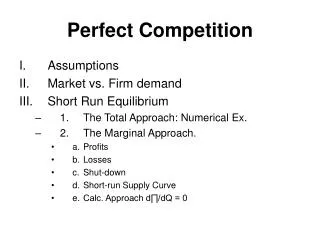
Perfect Competition in Market Economy
780 likes | 808 Views
This module explores Perfect Competition, its features, short-run price determination, and market morphology. Learn how firms operate in such markets and the equilibrium concepts regarding price, output levels, and profit maximization.

Perfect Competition in Market Economy
E N D
Presentation Transcript
Perfect Competition Prof. Nikhil Monga
OBJECTIVES • To understand market and market morphology • To understand Perfect Competition • To understand the features of Perfect Competition • To understand the short run price and output for the competitve industry and firm.
Market • Defined as the institutional relationship between buyers and sellers. • Market refers to the interaction between buyers and sellers of a good (or service) at a mutually agreed upon price. • Such interaction may be at a particular place, or may be over telephone, or even through the Internet! • Sellers and buyers may meet each other personally, or may not ever see each other, as in E-commerce. • Thus market may be defined as a place, a function, a process.
Markets may be characterized on the basis of: • Number, size and distribution of sellers in any market • Whether the product is homogeneous or differentiated • Number and size of buyers: • Freedom to enter into or exit from the market • Thus we have: • Perfect Competition • Monopoly • Monopolistic competition • Oligopoly
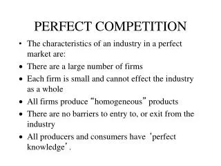
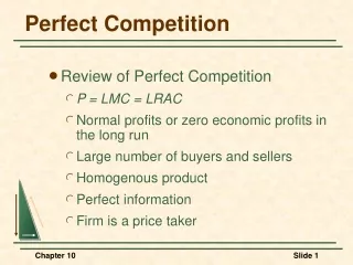
Features of Perfect Competition Perfect competition may be defined as that market where very large number of sellers sell homogeneous good to very large number of buyers while buyers and sellers have perfect knowledge of market conditions • Features • Presence of large number of buyers and sellers • Homogeneous product Eg Unbranded Spices • Freedom of entry and exit • Perfect knowledge • Perfectly elastic demand curve • Price determined by market and Firm is a price taker.
Price Taking The perfectly competitive firm is said to be a price-taker, because it takes the market price as given and has no control over the price. Why?...
If the firm tried to charge a higher price, it would lose all its business. Customers could go elsewhere to buy the same product for less. Since the firm is very small, it can sell as much as it wants at the market price. So there’s no reason to charge a lower price.
The demand curve for the product of the perfectly competitive firm shows how much can be sold at specific prices. Let’s see what it would look like... The firm can sell as little or as much as it wants at the market price. Suppose, for example, the market price is $5.
The firm can sell 10 units for $5. price $5 10 quantity
The firm can sell 20 units for $5. price $5 20 quantity
The firm can sell 30 units for $5. price $5 30 quantity
The firm can sell 40 units for $5. price $5 40 quantity
The firm can sell 50 units for $5. price $5 50 quantity
So all these points are on the demand curve for the firm’s product. price $5 quantity
Connecting these points, we have the demand curve for the firm’s product. price $5 demand quantity
The demand curve for the perfectly competitive firm’s product is a horizontal line at the market price. price market price demand quantity
Recall: Total Revenue Total Revenue = Price x Quantity TR = P Q
Recall: Marginal Revenue (MR) Marginal Revenue is the additional revenue earned from selling one additional unit of output. MR = DTR / DQ If MR>MC, we can increase total profit by producing more If MR<MC, we can increase profit by producing less Profit is maximum when MC=MR
Short run equilibrium of a firm • Over a short period, firm can face four situations as mentioned below • MR> ATC Supernormal Profit • MR= ATC Normal Profit • MR<ATC Losses • MR<ATC<AVC Shut down point MR stands for marginal revenue, ATC refers to average total cost and AVC stands for Average variable cost
The demand curve (D) and the MR curve for the perfectly competitive firm’s product. price market price D = MR quantity
Optimal Output Level To maximize profit, the firm will produce at the output level where MR = MC. So the firm will produce where the MR and MC curves intersect.
Costs C TFC O Quantity Costs TFC O Quantity Costs in Short Run • Fixed Costs • Do not vary with output; e.g. plant, machinery, building. • Total Fixed Cost (TFC) curve is a straight line, parallel to the quantity axis, indicating that output may increase to any level without causing any change in the fixed cost. • In the long run plant size may increase hence FC curve may be step like, where each step showing FC in a particular time period.
Average and Marginal Cost • Average Cost (AC) is total cost per unit of output. • AC is equal to the ratio of TC and units of output. (TC/Q) • AC=AFC+AVC • Average Fixed Cost (AFC) is fixed cost per unit of output (AFC= TFC/Q) • Average Variable Cost (AVC) is variable cost per unit of output (AVC= TVC/Q) • Marginal cost (MC) is the change in total cost due to a unit change in output. • MCQ= TCQ- TCQ-1 • Since the fixed component of cost cannot be altered, MC is virtually the change in variable cost per unit change in output. • Also known as rate of change in total cost.
MC AC/MC ATC AVC AFC O Quantity Average and Marginal Cost Functions Contd… • AC curve is U shaped • When both AFC and AVC fall, AC also falls and when AVC rises AC starts increasing. • When average costs decline, MC lies below AC. • When average costs are constant (at their minimum), MC equals AC. • MC passes through the lowest point of AC curves. • When average costs rise, MC curve lies above them.
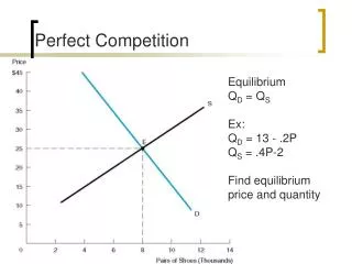
Price Price Market Demand Market Supply S D P=AR=MR E P* S D O O Output Output Q* Market Demand Curve and Firm’s Demand Curve • Market equilibrium is at the point of intersection (E) of the market demand and market supply curves, where equilibrium output for the industry is given at Q* and price at P*. • Each perfectly competitive firm, being a price taker, takes the equilibrium price from the market as given at P*. INDUSTRY FIRM
Short Run Price and Output for the Competitive Industry and Firm • In short run an individual firm may be in equilibrium and may earn • Supernormal profit: AR>AC • Normal profit: AR=AC • Losses: AR<AC
Price MC O Quantity Supernormal Profit • E is point of equilibrium as MC=MR and MC cut MR from below. At point E, MR>ATC & MR=AR • Firm is in equilibrium at OQ* output at market price P*, where both the conditions of equilibrium are fulfilled. • TR= OP*EQ* (TR= AR.Q) • TC= OABQ* (TC=AC.Q) • Profit = AP*EB = (OP*EQ*-OABQ*) • This is the supernormal profit made by the firm in the short run, because the market price P* (AR) is greater than average cost. MR>ATC ATC E P* AR=MR A B Q*
Price MC O Quantity Normal Profit • In the short run some firms may earn only normal profit (when average revenue is equal to average cost). E is point of equilibrium as MC=MR and MC cut MR from below. At point E, MR=ATC & MR=AR • Firm is in equilibrium at OQ* output at market price P*, where both the conditions of equilibrium are fulfilled. • TR= OP*EQ* • TC= OP*EQ* • TR=TC • Firm makes normal profit, and actually ends up producing at the break even level of output. AC=AR=MC=MR ATC E P* AR=MR Q*
Price ATC MC P* AR=MR O Quantity Losses • Firm is in equilibrium at OQ* output at market price P*, where both the conditions of equilibrium are fulfilled (point E). E is point of equilibrium as MC=MR and at equilibrium B>E, it implies AR<ATC and firm incur a loss of BE per unit of output produced. • TC= OABQ* • TR= OP*EQ* • Loss= P*ABE = OP*EQ* - OABQ* • The firm incurs loss or subnormal profit in the short run because the AC of producing this output is more than the market price hence TR<TC. • The firm continues to produce at loss in the short run in anticipation of price rise. AR<AC B A E Q*
Exit or Shut Down of Production AVC ATC Price MC O Quantity • A firm incurring losses in the short run will not withdraw from the market, but will wait for market conditions to improve in the long run. E is point of equilibrium as MC=MR, it produces Q amount of output, the firm incur average total cost of F, while it earns Average revenue E, At equilibrium F>E, the firm incur the loss of EF per unit of output produced. Since total earned revenue is OPEQ and total cost is ORFD. The loss is too much to continue, as this firm AVC is also above AR=MR so it should be shut down FIRM F R G AR=MR P* E Q*
Super normal Profit Normal Profit Losses Shut down point
Long Run Price and Output for the Industry and the Firm • In the long run perfectly competitive firms earn only normal profits. AR=MR=MC=AC • The reason is the unrestricted entry into and exit of firms from the industry in the long run. • When existing firms enjoy supernormal profits in the short run new firms are attracted to the industry to gain profits. • The supply of the commodity in the market increases. Assuming no change in the demand side, this lowers the price level. • When firms are making losses in the short run, some may be forced to leave the industry in the long run. • Their exit from the industry causes a reduction in the supply of the product and as a result the equilibrium price rises. • This process of adjustment continues up to the point where the price line becomes tangential to the AC curve.
Price LMC LAC P2 P1 AR=MR P* O Quantity Long Run Price and Output for the Industry and the Firm • Prevailing price is OP1, Equilibrium at Point E1 and Output OQ1 • Firms earn supernormal profit (AR>AC) • This will attract more firms, increase in supply will reduce the price till AC=AR, i.e. at P* • Prevailing price is OP2, Equilibrium at Point E2 and Output OQ2 • Firms earn loss (AR<AC) • Some firms will exit, decrease in supply will increase the price till AC=AR, i.e. at P* AR=MR=MC=AC E1 E* E2 Q1 Q2 Q*
MONOPOLY MONOPOLY
Introduction • A monopoly (from the Greek word “mono” meaning single and “polo” meaning to sell) is that form of market in which a single seller sells a product (good or service) which has no substitute. • Monopoly exists when there is no close substitute to the product and also when there is a single producer and seller of the product • E.g. Indian Railway is a monopoly, since there is no other agency in the country that provides railway service. • Pure monopoly is that market situation in which there is absolutely no substitute of the product, and the entire market is under control of a single firm. 37
Features • Single seller • The entire market is under control of a single firm. • Single product • A monopoly exists when a single seller sells a product which has no substitute or, at least, no close substitute in the market. • No difference between firm and industry • There is a single firm in the industry • Independent decision making • Firm is regarded as a price maker • Restricted entry • Existence of barriers leads to the emergence and/or survival of a monopoly 38
Types of Monopoly • Legal Monopoly • Created by the laws of a country in the greater public interest. • To prevent disparity in distribution of wealth, or imbalanced growth of the economy(State electricity Boards) • Economic Monopoly • Created due to superior efficiency of a particular player. • Technical know-how restrained in the hold of single • Control over scarce and key raw materials • Economies of Scale 39
Natural Monopoly • Size of the market is so small that it can accommodate only one player • Economies of Scale • Regional Monopoly • Geographical or territorial aspects also help in creation of monopolies.
Sources of Monopoly • Restriction by Law • Control over key Raw Materials • Specialized Know How • Economies of Large Scale • Small Market Size
Revenue, Cost AR MR O Quantity Demand and MR Curves • The demand curve of the monopolist is highly price inelastic because there is no close substitute and consumers have no or very little choice. • It is not perfectly inelastic because pure monopoly does not exist in real life. • Hence it faces a normal downward sloping demand (AR) curve. • MR curve corresponds. 42
Price, Revenue, Cost MC AC B PE A E AR MR O QE Quantity Price and Output Decisions in Short Run AR>AC • The monopolist cannot set both price and quantity at its own will. • In order to maximize profit a monopoly firm follows the rule of MR=MC when MC is rising. • A monopoly firm may earn supernormal profit or normal profit or even subnormal profit in the short run. • The negative slope of the demand curve is instrumental for chances of monopoly profits in the short run. • In the short run, the firm would reap the benefits of supplying a product which not only is unique, but also has negligible cross elasticity. 43
Price, Revenue, Cost Price, Revenue, Cost MC AC MC AC B A B PE PE C E AR E MR AR MR O Quantity O QE Quantity QE Price and Output Decisions in Short Run AR=AC AR<AC Total revenue= OPEBQE Total cost = OPEBQE Profit = Nil Firm makes normal profit. Total revenue= OPECQE Total cost = OABQE Loss = ABCPE Firm makes loss. 45
Price and Output Decisions in Long Run • It would try to reduce cost of production • Otherwise it would close down in the long run. • Monopolist would try to earn at least normal profit in the long run and may earn supernormal profit due to entry restrictions in the market. • If in the long run a monopoly firm earns supernormal profit • This would attract competition and high price would make it possible for a new entrant to survive. • To retain its monopoly power, the firm may have to resort to a low price and earn only normal profit even in the long run to create an economic barrier to new entrants. 46
Lecture Plan • Introduction • Features of Monopolistic Competition • Identification of industry • Demand and Marginal Revenue Curves of a Firm • Price and Output Decisions in Short Run • Price and Output Decisions in Long Run • Monopolistic Competition and Advertising • Comparison between Monopolistic Competition, Monopoly and Perfect Competition
Objectives • To understand the nature of imperfect competition or monopolistic competition. • To analyze the pricing and output decisions of a monopolistically competitive firm in the short run and long run.