Download
1 / 34
380 likes | 609 Views
Chapter 3 Steady-State Conduction -Multiple dimension. 3-1 Introduction. Differential eq. Fourier eq. 3-2 Mathematical analysis of two dimensional heat transfer. Problem : λ = const. No heat generation. The equation is linear homogeneous

E N D
Chapter 3 Steady-State Conduction -Multiple dimension
3-1 Introduction Differential eq. Fourier eq. 3-2 Mathematical analysis of two dimensional heat transfer Problem: λ= const. No heat generation
The equation is linear homogeneous All the boundaries are not homogeneous Set Substituting into governing eq. It is assumed that the may be separated into two functions in the form
For 2 <0 Not fit boundary condition excluded 2is separation const. For 2 =0 For 2 >0 Not fit boundary condition excluded
Applying boundary conditions n =1,2,3,……
From the 4th boundary condition To fit the boundary condition, n=1
If the 4th condition is (x,y)=f(x), no one of the n’s fits the boundary condition. We take the sum of this individual solutions as the general solution: From the 4th boundary conditions norm
If f(x)=T2, that is F(x)=T2- T1, then 3-3 Graphical analysis Self-learning
3-4 The conduction shape factor Plane wall Hollow cylinder General form Slab Hollow cylinder Other configuration: 2-D system with two limits of T
S is called shape factor, depends on geometry. For 3-D walls with all the interior dimension greater than 1/5
3-5 Numerical method of analysis General heat conduction problem There are two approaches to this problem 1. analytical method: 2. numerical method: Numerical heat transfer: the art of replacing the integrals or the partial derivatives in these equations with discretized algebraic forms, which in turn are solved to obtain numbers for the flow field values at discrete points in time and/or space. Continuous: a closed-form analytical solution variation of the dependent variables continuously through out the domain Discrete: a collection of numbers gives the answers at the discrete points in the domain
The procedure for numerical heat transfer • Mathematical models • Discretization of domain (node, grid) • Algebraic equations for all the nodes • Initial variable fields • Solving the algebraic equation • Analysis of the solution
y = ( k const ) = T T b b q x a 0 T h • Mathematical model 2-D problem
2. Discretization finite difference (有限差分) finite element (有限元法) boundary element (边界元法) finite analysis (有限分析法)
Grid generation Node(节点): discrete points control volume(控制容积): A properly selected region in space expressed by node Interface(界面): boundaries of control volume. Method for generating grid: practice A: the gridline generated first is to determine the nodes, then center is taken as the interface practice B: the gridline generated first is to determine the interface, then center is taken as the nodes Number of nodes: from 1 to N
+ m , n 1 , m + 1 n m , n - m 1 , n - m , n 1 3. Difference equations (1) Taylor series development at point (m, n) from eq.(1) First order (accurate) forward difference
from eq.(2) First order backward (rearward) difference (1)-(2) Second order central difference (1)+(2) Second order central second difference
Φn Φw Φe Φs In a similar way The finite difference approximation for the differential eq For uniform grid △x= △y , then (2)Heat balance Second order accuracy
(3) Boundary nodes The difference equations on boundary nodes depends on boundary conditions 1) For the first kind of boundary conditions Tb at y=b is known, no need for additional equations 2) For the first kind of boundary conditions, energy balance on node For uniform grid △x= △y , then
3) For the second kind of boundary conditions 4)once the temperature is determined, the heat flow is
4. Solution techniques • Direction solution method 直接求解 • matrix inversion 矩阵求逆 • elimination method 消元法 • large number of internal storage 内存大 • iteration method 迭代法 • Gauss—Seidel iteration • point iteration 点迭代 • line iteration 线迭代 • block iteration 块迭代 • widespread use 用得多
Nodal equations Matrix notation
The inverse of [A]-1 is The final solution is
5. Software packages for solution of equations MathCAD TK Solver Matlab Microsoft Excel
3-6 Numerical formulation in terms of resistance elements
3-7 Gauss---Seidel iteration Numerical formulation in terms of resistance elements φiis the the delivered to node i by heat generation Procedure • An initial set of values for the Ti zero value • Calculation of Ti always using the most recent values of the Tj Nodal equations: Rewritten : Superscript n is the iterations
End of the calculation when • is some selected constant accuracy of solution to the difference equations not the accuracy of solution to the physical problems
q rad, i Boit number For nodes with for x = yand no heat generation If Bi=0 the convective boundary is converted to insulated boundary Heat sources and boundary radiation exchange For radiation exchange at boundary node is the net radiation transferred to node I per unit area (chapter 8)
3-8 Accuracy considerations Two approaches to estimate the accuracy: • Compare the numerical solution with an analytical one Benchmark solution • Choose progressively smaller values of x and observe the behavior of the solution. T converge as x becomes smaller number of nodes round-off error Energy balance as check on solution accuracy Accuracy of properties and boundary conditions h 25% Uncertainties of surface radiation properties 10-300%
3-9 Electrical analogy for two-dimensional conduction self-learning 3-10 Summary self-learning


![Chapter 3: Unsteady State [ Transient ] Heat Conduction](https://cdn1.slideserve.com/2468294/chapter-3-unsteady-state-transient-heat-conduction-dt.jpg)