Download
1 / 56
560 likes | 721 Views
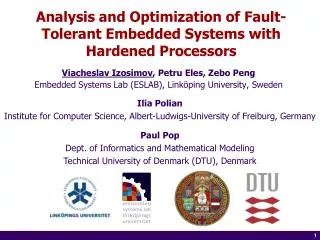
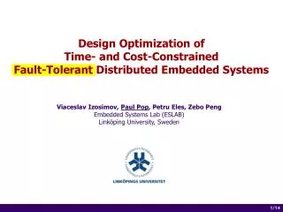
Presentation of Licentiate Thesis. Scheduling and Optimization of Fault-Tolerant Embedded Systems. Viacheslav Izosimov Embedded Systems Lab (ESLAB) Linköping University, Sweden. Motivation. Hard real-time applications Time-constrained Cost-constrained Fault-tolerant etc.

E N D
Presentation of Licentiate Thesis Scheduling and Optimization of Fault-Tolerant Embedded Systems Viacheslav IzosimovEmbedded Systems Lab (ESLAB)Linköping University, Sweden
Motivation • Hard real-time applications • Time-constrained • Cost-constrained • Fault-tolerant • etc. • Focus on transient faults and intermittent faults
Electromagnetic interference (EMI) Radiation Lightning storms Motivation Transient faults • Happen for a short time • Corruptions of data, miscalculation in logic • Do not cause a permanent damage of circuits • Causes are outside system boundaries
Transient faults Internal EMI Crosstalk Init (Data) Power supply fluctuations Software errors (Heisenbugs) Motivation Intermittent faults • Manifest similar as transient faults • Happen repeatedly • Causes are inside system boundaries
Motivation Transient faults are more likely to occuras the size of transistors is shrinkingand the frequency is growing Errors caused by transient faults haveto be tolerated before they crash the system However, fault tolerance againsttransient faults leads to significant performance overhead
The Need for Design Optimization of Embedded Systems with Fault Tolerance Motivation • Hard real-time applications • Time-constrained • Cost-constrained • Fault-tolerant • etc.
Outline • Motivation • Background and limitations of previous work • Thesis contributions: • Scheduling with fault tolerance requirements • Fault tolerance policy assignment • Checkpoint optimization • Trading-off transparency for performance • Mapping optimization with transparency • Conclusions and future work
Fault ToleranceTechniques Feedback loops General Design Flow System Specification Architecture Selection Mapping & Hardware / Software Partitioning Scheduling Back-end Synthesis
Error-detection overhead P1/2 P1 P1/1 P1 P1(1) N1 Recovery overhead P1(2) N2 Checkpointing overhead 40 20 0 60 N1 N1 P1 1 P1 2 P1 P1 1 1 P1 P1 2 2 P1/2 P1/1 2 2 N1 N1 P1(1) N2 P1(2) Fault Tolerance Techniques Re-execution N1 Rollback recovery with checkpointing P1 1 Active replication
Limitations of Previous Work • Design optimization with fault tolerance is limited • Process mapping is not considered together with fault tolerance issues • Multiple faults are not addressed in the framework of static cyclic scheduling • Transparency, if at all addressed, is restricted to a whole computation node
Outline • Motivation • Background and limitations of previous work • Thesis contributions: • Scheduling with fault tolerance requirements • Fault tolerance policy assignment • Checkpoint optimization • Trading-off transparency for performance • Mapping optimization with transparency • Conclusions and future work
Transient faults Processes: Re-execution,Active Replication, RollbackRecovery with Checkpointing Messages: Fault-tolerant predictable protocol P5 m2 m1 P1 P2 P3 P4 Fault-Tolerant Time-Triggered Systems … Maximum k transient faults within each application run (system period)
Conditional Scheduling Scheduling with Fault Tolerance Reqirements Conditional Scheduling Shifting-based Scheduling
P1 m1 P2 k = 2 Conditional Scheduling P1 0 20 40 60 80 100 120 140 160 180 200
P1 m1 P2 k = 2 Conditional Scheduling P1 P2 0 20 40 60 80 100 120 140 160 180 200
P1/1 P1/2 P1 m1 P2 k = 2 Conditional Scheduling P1 0 20 40 60 80 100 120 140 160 180 200
P1 m1 P2 k = 2 Conditional Scheduling P1/1 P1/2 P1/3 P2 0 20 40 60 80 100 120 140 160 180 200
P2/1 P2/2 P1 m1 P2 k = 2 Conditional Scheduling P1/1 P1/2 P2 0 20 40 60 80 100 120 140 160 180 200
P2/1 P2/2 P2/3 P1 m1 P2 k = 2 Conditional Scheduling P1 P2 0 20 40 60 80 100 120 140 160 180 200
k = 2 Conditional Scheduling Fault-Tolerance Conditional Process Graph P1 1 m1 1 P1 2 P2 1 P1 m1 2 P1 3 m1 P2 P2 4 2 m1 3 P2 P2 P2 P2 6 3 5
N1 N2 k = 2 Conditional Schedule Table P1 m1 P2
Conditional Scheduling • Conditional scheduling: • Generates short schedules • Allows to trade-off between transparency and performance (to be discussed later...) • Requires a lot of memory to store schedule tables • Scheduling algorithm is very slow • Alternative: shifting-based scheduling
Shifting-based Scheduling • Messages sent over the bus should be scheduled at one time • Faults on one computation node must not affect other computation nodes • Requires less memory • Schedule generation is very fast • Schedules are longer • Does not allow to trade-off between transparency and performance (to be discussed later...)
P1 1 P2 P1 1 2 P2 4 P2 P1 2 3 P2 5 P2 P2 3 6 m2 m1 S m3 S P2 after P1 S k = 2 P1 m2 P4 1 m1 P4 P2 P3 P4 1 2 m3 P3 P3 4 2 P3 after P4 P3 P4 3 P3 3 P3 P3 5 5 Ordered FT-CPG
Recovery slack for P1 andP2 P1 P1 Worst-case scenario for P1 Root Schedules P2 P1 N1 P3 P4 N2 m2 m3 m1 Bus
Extracting Execution Scenarios P1 P2 N1 P3 P4/3 P4/2 P4/1 N2 m2 m3 m1 Bus
1.73 4.96 8.09 12.56 16.72 Memory Required to Store Schedule Tables • Applications with more frozen nodesrequire less memory
0.03 1.73 Memory Required to Store Root Schedule • Shifting-based scheduling requires very little memory
Schedule Generation Time and Quality Shifting-based scheduling requires 0.2 seconds to generate a root schedule for application of 120 processes and 10 faults Conditional scheduling already takes 319 seconds to generate a schedule table for application of 40 processes and 4 faults • Shifting-based scheduling much faster thanconditional scheduling ~15% worse than conditional scheduling with100% inter-processor messages set to frozen (in terms of fault tolerance overhead)
Fault Tolerance Policy Assignment Checkpoint Optimization
2 N1 P1(1) N1 P1(1)/1 P1(1)/2 N2 P1(2) P1(2) N2 N3 P1(3) Re-executed replicas Replication Fault Tolerance Policy Assignment N1 P1/1 P1/2 P1/3 Re-execution
Deadline Deadline N1 P1(1) P2(1) P3(1) Missed N1 P1(1) P2(1) P3(1) P1 N2 P1(2) P2(2) P3(2) Met N2 P1(2) P2(2) P3(2) m1 P3 P2 bus bus m2(1) m1(1) m2(2) m1(2) m1(1) m1(2) N1 P1 P2 P3 N1 P1 P2 Met Missed N2 N2 P3 N1 N2 bus N1 N2 bus P1 40 50 P2 40 50 P3 60 70 1 Re-execution vs. Replication Re-execution is better Replication is better m2 m1 P1 P2 P3 A2 A1
Deadline 1 N1 P1 P2 P4 N1 N2 N2 P3 Missed P1 40 50 P2 60 80 P3 60 80 bus P4 40 50 m2 N1 N2 m2 P3 m3 P1 m1 P2 P4 Optimizationof fault tolerancepolicy assignment N1 P1(1) P2 P4 Met N2 P1(2) P3 bus m1(2) m2(1) N1 P1(1) P2(1) P3(1) P4(1) Missed N2 P1(2) P2(2) P3(2) P4(2) bus m1(1) m1(2) m2(1) m2(2) m3(1) m3(2) Fault Tolerance Policy Assignment
Optimization Strategy • Design optimization: • Fault tolerance policy assignment • Mapping of processes and messages • Root schedules • Three tabu-search optimization algorithms: • Mapping and Fault Tolerance Policy assignment (MRX) • Re-execution, replication or both • Mapping and only Re-Execution (MX) • Mapping and only Replication (MR) Tabu-search Shifting-based scheduling
Mapping and replication (MR) 80 Mapping and re-execution (MX) 20 Experimental Results Schedulability improvement under resource constraints 100 90 80 70 60 Avgerage % deviation from MRX 50 40 30 20 10 Mapping and policy assignment (MRX) 0 20 40 60 80 100 Number of processes
P1/1 P1 P1 P1 P1 P1 P1 P1/2 2 2 1 1 2 2 2 2 N1 Checkpoint Optimization P1
P1 1 1 2 P1 P1 2 1 2 3 P1 P1 P1 3 1 2 3 4 P1 P1 P1 P1 4 1 2 3 4 5 5 P1 P1 P1 P1 P1 Locally Optimal Number of Checkpoints k = 2 c1 = 5 ms No. of checkpoints a1 = 10 ms 1= 15 ms C1 = 50 ms P1
1 2 3 P1 P1 P1 1 2 3 1 2 1 2 P2 P2 P2 P1 P1 P2 P2 265 255 Globally Optimal Number of Checkpoints k = 2 C1 = 50 ms P1 c a m1 P1 10 10 5 P1 P2 P2 C2=60 ms P2 10 5 10
Globally Optimal Number of Checkpoints 265 1 2 3 1 2 3 a) P1 P1 P1 P2 P2 P2 255 1 2 1 2 b) P1 P1 P2 P2 k = 2 C1 = 50 ms P1 c a m1 P1 10 10 5 P1 P2 P2 C2=60 ms P2 10 5 10
Globally Optimal Number of Checkpoints 265 1 2 3 1 2 3 a) P1 P1 P1 P2 P2 P2 255 1 2 1 2 b) P1 P1 P2 P2 k = 2 C1 = 50 ms P1 c a m1 P1 10 10 5 P1 P2 P2 C2=60 ms P2 10 5 10
Does the optimization reduce the fault tolerance overheads on the schedule length? 40% 30% 4 nodes, 3 faults % deviation from MC0 (how smaller the fault tolerance overhead) 20% Global Optimization of Checkpoint Distribution (MC) 10% Local Optimization of Checkpoint Distribution (MC0) 0% 40 60 80 100 Application size (the number of tasks) Global Optimization vs. Local Optimization
Trading-off Transparency for Performance Mapping Optimization with Transparency
– regular processes/messages – frozen processes/messages P3 Frozen Transparency is achieved with frozen processes and messages Good for debugging and testing FT Implementations with Transparency P5 m2 m1 P1 P2 P3 P4 Performance overhead!
processes start at different times no fault scenario P1 P2 N1 N2 messages are sent at different times P1 30 X P4 P3 P2 20 X P3 X 20 P4 X 30 m2 m1 m3 the worst-case fault scenario N1 P1 P1 P2 N2 P4 P4 P3 k = 2 bus m2 m1 m3 P1 P2 m2 m3 m1 P3 P4 No Transparency Deadline N1 N2 bus = 5 ms N1 N2
No transparency P1 P1 P2 P4 P4 P3 m2 m1 m3 Full transparency P2 P1 P4 P3 P3 P3 m2 m1 m3 P2 P1 no fault scenario P4 P3 Customized transparency P1 P2 m2 m1 m3 P4 P3 P3 P3 m1 m3 m2 P1 P1 P2 P1 P4 P3 m2 m1 m3 Full Transparency Customized Transparency Deadline Deadline
How longer is the schedule length with fault tolerance? 29 40 49 60 66 Trading-Off Transparency for Performance increasing transparency • Trading transparency for performance is essential Four (4) computation nodes Recovery time 5 ms
optimal mapping without transparency P4 P2 P5 P1 P3 P6 N1 P4/1 P4/2 P4/3 P5 P2 the worst-case fault scenario for optimal mapping N2 P1 P3 P6 N1 N2 k = 2 bus P1 30 30 m1 40 40 P2 P3 50 50 P4 60 60 P5 40 40 P6 50 50 Mapping with Transparency Deadline N1 N2 bus m1 P1 m1 m2 = 10 ms N1 N2 P3 P4 P2 m4 m3 P5 P6
P1 m1 m2 P4 P2/2 P2/1 P2/3 P5 P3 P4 P2 P1 P3 P6 m4 m3 P5 P6 the worst-case fault scenario with transparency and optimized mapping N1 P1 P2 P5 N2 P4/1 P3 P4/2 P4/3 P6 N1 N2 k = 2 P1 30 30 bus m2 40 40 P2 P3 50 50 P4 60 60 P5 40 40 P6 50 50 Mapping with Transparency Deadline N1 the worst-case fault scenario with transparency for “optimal” mapping N2 bus m1 = 10 ms N1 N2
Design Optimization Hill-climbing mapping optimization heuristic Schedule length 1. Conditional Scheduling (CS) Slow 2. Schedule Length Estimation (SE) Fast
How faster is schedule length estimation (SE) compared to conditional scheduling (CS)? Experimental Results 318.88s 0.69s Schedule length estimation (SE) is more than 400 times faster than conditional scheduling (CS)