Download
1 / 18
180 likes | 299 Views
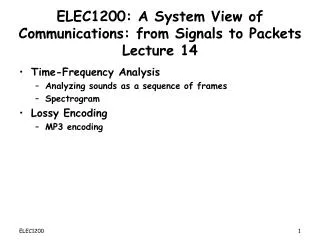
ELEC1200: A System View of Communications: from Signals to Packets Lecture 14. Time-Frequency Analysis Analyzing sounds as a sequence of frames Spectrogram Lossy Encoding MP3 encoding. Time-Frequency Analysis.

E N D
ELEC1200: A System View of Communications: from Signals to PacketsLecture 14 • Time-Frequency Analysis • Analyzing sounds as a sequence of frames • Spectrogram • Lossy Encoding • MP3 encoding
Time-Frequency Analysis • For many complex signals (like speech, music and other sounds), short segments are well described by a sinusoidal representation with a few important frequency components, but long segments are not. • Time-frequency analysis refers to the analysis of how short-term frequency content changes over time. • The spectrogram of a signal is a picture of how its amplitude spectrum of a signal changes over time. • The vertical axis represents frequency • The horizontal axis represents time • The image color represents Fourier amplitude • red = large amplitude, blue = small amplitude
amplitude spectrum 35 loud many frequencies 30 25 amplitude spectrum 20 35 quiet lower frequency 15 30 10 25 5 20 0 15 0 1000 2000 3000 4000 frequency (Hz) 10 5 0 0 1000 2000 3000 4000 frequency (Hz) Spectrogram Example amplitude spectrum 35 loud high frequency 30 25 20 15 10 5 0 0 1000 2000 3000 4000 frequency (Hz) 4000 blue = quiet red = loud 3500 3000 2500 frequency (Hz) 2000 1500 1000 500 0 5 10 15 20 25 30 35 frame number
Computation of the Spectrogram • Divide the signal into a set of frames, typically about 20-50ms long. • Compute the amplitude spectrum of each frame. • This gives you a two dimensional array of real numbers, indexed by frame number and frequency index. • Plot this as an image. • It is generally more informative to plot the logarithm of the amplitude, as this compresses large amplitudes allowing the smaller details to show up. • To avoid problems at zero, apply a small positive floor to the values (i.e. replace each amplitude by P if it is smaller than P, where P is small). frame
Speech Spectrogram spectrogram of “she” can you guess what word this is? 4000 4000 3500 3500 3000 3000 2500 2500 frequency (Hz) frequency (Hz) 2000 2000 1500 1500 1000 1000 500 500 0 0 5 10 15 20 25 30 35 5 10 15 20 25 30 35 frame number frame number
Train Whistle vs. Bird Chirps • Can you figure out which is which? spectrogram spectrogram 4000 4000 3500 3500 3000 3000 2500 2500 frequency (Hz) frequency (Hz) 2000 2000 1500 1500 1000 1000 500 500 0 0 10 20 30 40 50 10 20 30 40 50 frame number frame number
Speech Data red = high energy blue = low energy • Characteristics • Recent measurements more informative in predicting the future than those in the distant past. • At each point in time, different sounds (phonemes) may be pronounced. • Different phonemes have different spectral content. phonemes
Encoding and Decoding • Encoding • Auditory signal (from a recording) is coded into an mp3 file containing carefully stored spectral information • Decoding • mp3 file is turned back into an auditory file that can be output to your speakers Source Encoding Source Decoding Store/Retrieve Transmit/Receive bitsIN bitsOUT
Lossless vs. Lossy Compression Source Encoding Source Decoding • For losslessdata compression: bitsOUT = bitsIN • We can reconstruct the original bit stream exactly • bitsOUT= bitsIN • Usually used for “naturally digital” bit streams, e.g. documents, messages, datasets, … • Examples: Huffman encoding, LZW, zip files, rar files • For lossyencodings: bitsOUT ≈ bitsIN • “Essential” information preserved • Appropriate for sampled data streams (audio, video) intended for human consumption via imperfect sensors (ears, eyes). Store/Retrieve Transmit/Receive bitsIN bitsOUT
MP3 • MPEG is moving pictures experts group • set up by ISO (international standards organization) • every few years issues a standard • MPEG1 (1992) • MPEG2(1994).. • MP3 stands for MPEG audio layer III • MP3 achieves a 10:1 compression ratio! • This enables • bit-streaming • compact audio storage
Bad ways to compress an audio file • Reduce the total number of bits per sample • e.g. 32 bit to 16 or 16 to 8 bit • Gives you a factor of 2 in compression • However, perceptual quality of signal is poor • Reduce the sampling rate • 44kHz to 22kHz or 22kHz to 10kHz • Again only a gain of a factor of 2 in size. • Total loss of all high frequency information. • Equivalent to a high pass filter. • A factor 10:1 in compression cannot be achieved using linear compression schemes
Perceptual Coding • Start by evaluating input response of bitstream consumer (eg, human ears or eyes), i.e., how consumer will perceive the input. • Frequency range, amplitude sensitivity, color response, … • Masking effects • Identify information that can be removed from bit stream without perceived effect, e.g., • Sounds outside frequency range • Masked sounds • Encode remaining information efficiently • Use frequency-based transformations • Quantize coefficients of frequency (loss occurs here) • Add lossless coding (e.g. the Huffman encoding to be studied later)
Principles of Auditory Coding • Time frequency decomposition • divide the signal into frames • obtain the spectrum of each piece • Use psycho-acoustic model to determine what information to keep • Don’t store information outside the range of hearing (40Hz to 15kHz) • Stereo info not stored for low frequencies • Masking • Store the information in the most compact way possible • minimize the bitrate • maximize the audible auditory content
Masking • If a dominant tone is present then noise can be added at frequencies next to it and this noise will not be heard. • Coding consequences • Less precision is required to store nearby frequencies • Less precision = coarser quantization • Definitions • Auditory threshold – minimum signal level at which a pure tone can be heard • Masking threshold – minimum signal level if a dominant tone is present
MP3 schematic • Input: 16 bit at 44kHz sampling is 768kbit/s • Output: Coded audio signal at ~128kbit/s lossless compression to be studied later Frequency analysis similar to Fourier series loss of information happens here minor extra information encoded here Frequency analysis similar to Fourier series effects of masking determined here
Quantization • When creating a digital representation of a sampled value, we must choose the number of bits used to represent the value. • Since fewer bits encode a smaller number of values, using fewer bits results in a larger quantization error • quantization error = difference between the actual and encoded value • We want quantization error to be small, i.e. more bits. • On the other hand, fewer bits take up less space. sixteen possible values eight possible values four possible values quantization error
Non-uniform quantization • MP3 compression quantizes the amplitudes of different frequency components differently, depending upon masking. • Frequency components near a dominant masker are quantized with lower bits. lossless compression to be studied later Frequency analysis similar to Fourier series loss of information happens here minor extra information encoded here Frequency analysis similar to Fourier series effects of masking determined here
Summary • Audio waveforms are typically analyzed as a sequence of frames • Within each frame, the signal can be well approximated by a few frequency components • The spectrogram can be used to visualize changes in the frequency content over time • Framing is used in MP3 audio compression • MP3 audio compression combines framing and frequency analysis with a non-uniform quantization based on a perceptual model • Quantization results in loss of information • By throwing away “unimportant” (imperceptible) information, we can obtain large compression ratios. • We will study a very simple version of this idea in the lab.