Download
1 / 127
1.72k likes | 2.97k Views
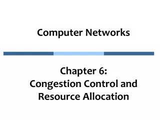
Computer Networks Chapter 6: Congestion Control and Resource Allocation. Problem. We have seen enough layers of protocol hierarchy to understand how data can be transferred among processes across heterogeneous networks Problem

E N D
Computer NetworksChapter 6: Congestion Control and Resource Allocation
Problem • We have seen enough layers of protocol hierarchy to understand how data can be transferred among processes across heterogeneous networks • Problem • How to effectively and fairly allocate resources among a collection of competing users?
Chapter Outline • Issues in Resource Allocation • Queuing Disciplines • TCP Congestion Control • Congestion Avoidance Mechanism • Quality of Service
6.1 Congestion Control and Resource Allocation • Resources • Bandwidth of the links • Buffers at the routers and switches • Packets contend at a router for the use of a link, with each contending packet placed in a queue waiting for its turn to be transmitted over the link
Congestion Control and Resource Allocation • When too many packets are contending for the same link • The queue overflows • Packets get dropped • Network is congested! • Network should provide a congestion control mechanism to deal with such a situation
Congestion Control and Resource Allocation • Congestion control and Resource Allocation • Two sides of the same coin • If the network takes active role in allocating resources • The congestion may be avoided • No need for congestion control
Congestion Control and Resource Allocation • Allocating resources with any precision is difficult • Resources are distributed throughout the network • On the other hand, we can always let the sources send as much data as they want • Then recover from the congestion when it occurs • Easier approach but it can be disruptive because many packets may be discarded by the network before congestions can be controlled
Congestion Control and Resource Allocation • Congestion control and resource allocations involve both hosts and network elements such as routers • In network elements (Routers) • Various queuing disciplines can be used to control the order in which packets get transmitted and which packets get dropped • At the hosts’ end • The congestion control mechanism paces how fast sources are allowed to send packets
Issues in Resource Allocation • Network Model • Packet Switched Network • A packet-switched network (or internet) consisting of multiple links and switches (or routers) is considered. • A given source may have more than enough capacity on the immediate outgoing link to send a packet, but somewhere in the middle of a network, its packets encounter a link that is being used by many different traffic sources
Issues in Resource Allocation • Network Model • Packet Switched Network A potential bottleneck router.
Issues in Resource Allocation • Network Model • Connectionless Flows • Assume that the network is connectionless (IP), with any connection-oriented service (TCP) implemented in the transport protocol that is running on the end hosts. • Datagrams are switched independently • But it is usually the case that a stream of datagrams between a particular pair of hosts flows through a particular set of routers
Issues in Resource Allocation • Network Model • Connectionless Flows Multiple flows passing through a set of routers
Issues in Resource Allocation • Network Model • Connectionless Flows • Flows can be defined at different granularities. • For example, a flow can be host-to-host or process-to-process. • In the latter case, a flow is essentially the same as a channel. • A flow is visible to the routers inside the network, whereas a channel is an end-to-end abstraction.
Issues in Resource Allocation • Network Model • Connectionless Flows • Because multiple related packets flow through each router, it sometimes makes sense to maintain some state information for each flow, which can be used to make resource allocation decisions about the packets that belong to the flow. • This state is sometimes called soft state. • The main difference between soft state and “hard” state is that soft state needs not always be explicitly created and removed by signalling.
Issues in Resource Allocation • Network Model • Connectionless Flows • Soft state represents a middle ground between • a purely connectionless network that maintains no state at the routers and • a purely connection-oriented network that maintains hard state at the routers. • Each packet is still routed correctly without regard to this state, but when a packet happens to belong to a flow for which the router is currently maintaining soft state, then the router is better able to handle the packet.
Issues in Resource Allocation • Taxonomy • Router-centric versus Host-centric • In a router-centric design, each router takes responsibility for • deciding when packets are forwarded • selecting which packets are to dropped, • informing the hosts how many packets they are allowed to send. • In a host-centric design, the end hosts observe the network conditions and adjust their behavior accordingly. • They are not mutually exclusive.
Issues in Resource Allocation • Taxonomy • Reservation-based versus Feedback-based • In a reservation-based system, the end host asks the network for a certain amount of capacity to be allocated for a flow. • Each router then allocates enough resources (buffers and/or percentage of the link’s bandwidth) to satisfy this request. • If the request cannot be satisfied at some router, then the reservation is rejected.
Issues in Resource Allocation • Taxonomy • Reservation-based versus Feedback-based • In a feedback-based approach, the end hosts begin sending data without first reserving any capacity and then adjust their sending rate according to the feedback they receive. • This feedback can either be • explicit (i.e., a congested router sends a “please slow down” message to the host) • or it can be implicit (i.e., the end host adjusts its sending rate according to the externally observable behavior of the network, such as packet losses).
Issues in Resource Allocation • Taxonomy • Window-based versus Rate-based • Window advertisement is used within the network to reserve buffer space. • Control sender’s behavior using a rate, how many bit per second the receiver or network is able to absorb.
Issues in Resource Allocation • Evaluation Criteria • Effective Resource Allocation • Evaluating the effectiveness of a resource allocation scheme is to consider the two principal metrics of networking: throughput and delay. • As much throughput and as little delay as possible. • To increase throughput Allow as many packets into the network as possible, so as to drive the utilization of all the links up to 100%. • But this also increases the queue length at each router. • Packets are delayed longer in the network
Issues in Resource Allocation • Evaluation Criteria • Effective Resource Allocation • The ratio of throughput to delay is used as a metric for evaluating the effectiveness of a resource allocation scheme. • This ratio is sometimes referred to as the power of the network. • Power = Throughput/Delay
Issues in Resource Allocation • Evaluation Criteria • Effective Resource Allocation Ratio of throughput to delay as a function of load
Issues in Resource Allocation • Evaluation Criteria • Fair Resource Allocation • The issue of fairness needs also be considered. • For example, a reservation-based resource allocation scheme provides an explicit way to create controlled unfairness. • With such a scheme, we might use reservations to enable a video stream to receive 1 Mbps across some link while a file transfer receives only 10 Kbps over the same link.
Issues in Resource Allocation • Evaluation Criteria • Fair Resource Allocation • Without explicit information, when several flows share a particular link, we would like for each flow to receive an equal share of the bandwidth. • This definition presumes that a fair share of bandwidth means an equal share of bandwidth. • But even without reservations, equal shares may not equate to fair shares. • Should we also consider the length of the paths being compared ?
Issues in Resource Allocation • Evaluation Criteria • Fair Resource Allocation One four-hop flow competing with three one-hop flows
Issues in Resource Allocation • Evaluation Criteria • Fair Resource Allocation • Assuming that fair implies equal and that all paths are of equal length, networking researcher Raj Jain proposed a metric that can be used to quantify the fairness of a congestion-control mechanism. • Jain’s fairness index is defined as follows. Given a set of flow throughputs (x1, x2, . . . , xn) (measured in consistent units such as bits/second), the following function assigns a fairness index to the flows: • The fairness index always results in a number between 0 and 1, with 1 representing greatest fairness.
6.2 Queuing Disciplines • The idea of FIFO queuing, also called first-come-first-served (FCFS) queuing, is simple: • The first packet that arrives at a router is the first packet to be transmitted • Assume the buffer space is finite. If a packet arrives and the queue is full, then the router discards that packet • Tail drop, since packets that arrive at the tail end of the FIFO are dropped • Note that tail drop and FIFO are two separable ideas. FIFO is a scheduling discipline—it determines the order in which packets are transmitted. Tail drop is a drop policy—it determines which packets get dropped
Queuing Disciplines (a) FIFO queuing; (b) tail drop at a FIFO queue.
Queuing Disciplines • Priority Queuing • A simple variation on basic FIFO queuing. • The idea is to mark each packet with a priority; the mark could be carried in the IP header. • The routers then implement multiple FIFO queues, one for each priority class. The router always transmits packets out of the highest-priority queue if that queue is nonempty before moving on to the next priority queue. • Within each priority, packets are still managed in a FIFO manner.
Queuing Disciplines • Fair Queuing • The main problem with FIFO queuing is that it does not discriminate between different traffic sources, or it does not separate packets according to the flow to which they belong. • Fair queuing (FQ) maintains a separate queue for each flow currently being handled by the router. • The router then services these queues in a sort of round-robin
Queuing Disciplines • Fair Queuing Round-robin service of four flows at a router
Queuing Disciplines • Fair Queuing • The main complication with Fair Queuing is that the packets being processed at a router are not necessarily the same length. • To truly allocate the bandwidth of the outgoing link in a fair manner, it is necessary to take packet length into consideration. • For example, if a router is managing two flows with round-robin scheduling: • 1st flow: 1000-byte packets 2/3 bandwidth • 2nd flow: 500-byte packets 1/3 bandwidth
Queuing Disciplines • Fair Queuing • What we really want is bit-by-bit round-robin the router transmits a bit from flow 1, then a bit from flow 2, and so on. • This is not feasible !! • The FQ mechanism simulates this behavior: • First, determining when a given packet would finish being transmitted if it was being sent using bit-by-bit round-robin • Then using this finishing time to sequence the packets for transmission.
Queuing Disciplines • Fair Queuing • To understand the algorithm for approximating bit-by-bit round robin, consider the behavior of a single flow • For this flow, let • Pi : denote the length of packet i • Si: time when the router starts to transmit packet i • Fi: time when router finishes transmitting packeti • Clearly, Fi = Si + Pi
Queuing Disciplines • Fair Queuing • When do we start transmitting packet i? • Depends on whether packetiarrived before or after the router finishes transmitting packet i-1 for the flow • Let Ai denote the time that packet i arrives at the router • Then Si = max(Fi-1, Ai) • Fi = max(Fi-1, Ai) + Pi
Queuing Disciplines • Fair Queuing • Now for every flow, we calculate Fi for each packet that arrives using our formula • We then treat all the Fias timestamps • Next packet to transmit is always the packet that has the lowest timestamp • The packet that should finish transmission before all others
Queuing Disciplines • Fair Queuing Example of fair queuing in action: packets with earlier finishing times are sent first; sending of a packet already in progress is completed
6.3 TCP Congestion Control • TCP congestion control was introduced into the Internet in the late 1980s by Van Jacobson, roughly eight years after the TCP/IP protocol stack had become operational. • Immediately preceding this time, the Internet was suffering from congestion collapse — • hosts would send their packets into the Internet as fast as the advertised window would allow, congestion would occur at some router (causing packets to be dropped), and the hosts would time out and retransmit their packets, resulting in even more congestion
TCP Congestion Control • The idea of TCP congestion control is for each source to determine how much capacity is available in the network, so that it knows how many packets it can safely have in transit. • Once a given source has this many packets in transit, it uses the arrival of an ACK as a signal that one of its packets has left the network, and that it is therefore safe to insert a new packet into the network without adding to the level of congestion. • By using ACKs to pace the transmission of packets, TCP is said to be self-clocking.
TCP Congestion Control • Additive Increase Multiplicative Decrease (AIMD) • TCP maintains a new state variable for each connection, called CongestionWindow, which is used by the source to limit how much data it is allowed to have in transit at a given time. • The congestion window is congestion control’s counterpart to flow control’s advertised window. • TCP is modified such that the maximum number of bytes of unacknowledged data allowed is now the minimum of the congestion window and the advertised window
TCP Congestion Control • Additive Increase Multiplicative Decrease (AIMD) • TCP’s effective window is revised as follows: • MaxWindow = MIN (CongestionWindow, AdvertisedWindow) • EffectiveWindow = MaxWindow − (LastByteSent − LastByteAcked). • That is, MaxWindow replaces AdvertisedWindow in the calculation of EffectiveWindow. • A TCP source is allowed to send no faster than the slowest component—the network or the destination host—can accommodate.
TCP Congestion Control • Additive Increase Multiplicative Decrease (AIMD) • How TCP comes to learn an appropriate value for CongestionWindow? • The AdvertisedWindow is sent by the receiving side of the connection. • But no one to send a suitable CongestionWindow to the sending side of TCP. • TCP source sets the CongestionWindow based on the level of congestion it perceives to exist in the network. • Decreasing the congestion window when the level of congestion goes up and increasing the congestion window when the level of congestion goes down. • Called additive increase/multiplicative decrease (AIMD)
TCP Congestion Control • Additive Increase Multiplicative Decrease (AIMD) • How does the source determine that the network is congested and that it should decrease the congestion window? • TCP interprets timeouts as a sign of congestion and reduces the rate at which it is transmitting. • Specifically, each time a timeout occurs, the source sets CongestionWindow to half of its previous value. • This halving of the CongestionWindow for each timeout corresponds to the “multiplicative decrease” part of AIMD.
TCP Congestion Control • Additive Increase Multiplicative Decrease (AIMD) • Although CongestionWindow is defined in terms of bytes, it is easiest to understand multiplicative decrease if we think in terms of whole packets. • For example, suppose the CongestionWindow is currently set to 16 packets. If a loss is detected, CongestionWindow is set to 8. • Additional losses cause CongestionWindow to be reduced to 4, then 2, and finally to 1 packet. • CongestionWindow is not allowed to fall below the size of a single packet, or in TCP terminology, the maximum segment size (MSS).
TCP Congestion Control • Additive Increase Multiplicative Decrease (AIMD) • A congestion-control strategy that only decreases the window size is obviously too conservative. • We also need to be able to increase the congestion window to take advantage of newly available capacity in the network. • This is the “additive increase” part of AIMD, and it works as follows. • Every time the source successfully sends a CongestionWindow’s worth of packets—that is, each packet sent out during the last RTT has been ACKed—it adds the equivalent of 1 packet to CongestionWindow.
TCP Congestion Control • Additive Increase Multiplicative Decrease (AIMD) Packets in transit during additive increase, with one packet being added each RTT.
TCP Congestion Control • Additive Increase Multiplicative Decrease (AIMD) • Note that in practice, TCP does not wait for an entire window’s worth of ACKs to add 1 packet’s worth to the congestion window, but instead increments CongestionWindow by a little for each ACK that arrives. • Specifically, the congestion window is incremented as follows each time an ACK arrives: • Increment = MSS × (MSS/CongestionWindow) • CongestionWindow+= Increment • That is, rather than incrementing CongestionWindow by an entire MSS bytes each RTT, we increment it by a fraction of MSS every time an ACK is received. • Assuming that each ACK acknowledges the receipt of MSS bytes, then that fraction is MSS/CongestionWindow.
TCP Congestion Control • Slow Start • The additive increase mechanism just described is the right approach to use when the source is operating close to the available capacity of the network, but it takes too long to ramp up a connection when it is starting from scratch. • TCP therefore provides a second mechanism, ironically called slow start, that is used to increase the congestion window rapidly from a cold start. • Slow start effectively increases the congestion window exponentially, rather than linearly.
TCP Congestion Control • Slow Start • Specifically, the source starts out by setting CongestionWindow to one packet. • When the ACK for this packet arrives, TCP adds 1 to CongestionWindow and then sends two packets. • Upon receiving the corresponding two ACKs, TCP increments CongestionWindow by 2—one for each ACK—and next sends four packets. • The end result is that TCP effectively doubles the number of packets it has in transit every RTT.
TCP Congestion Control • Slow Start Packets in transit during slow start.