Download
1 / 34
340 likes | 538 Views
Current and Future SZ Surveys. Sunil Golwala California Institute of Technology July 7, 2001. Overview. The Sunyaev-Zeldovich effect in galaxy clusters Science with blind SZE surveys Interferometers and bolometer arrays Calculating expected sensitivities

E N D
Current and Future SZ Surveys Sunil Golwala California Institute of Technology July 7, 2001
Overview • The Sunyaev-Zeldovich effect in galaxy clusters • Science with blind SZE surveys • Interferometers and bolometer arrays • Calculating expected sensitivities • Laundry list of current and future instruments: specifications and sensitivities • Summary for the near future • Thanks to all the instrument teams for specs and numbers!
The Sunyaev-Zeldovich Effect in Galaxy Clusters • Thermal SZE is the Compton up-scattering of CMB photons by electrons in hot, intracluster plasma CMB photons T = (1 + z) 2.725K ∆TCMB/TCMB depends only on cluster y ~ line-of-sight integral of neTe. Both ∆TCMBand TCMB are redshifted similarly ratio unchanged as photons propagate and independent of cluster distance galaxy cluster with hot ICM z ~ 0 - 3 scattered photons (hotter) observer z = 0 last scatteringsurface z ~ 1100 thermal SZE causes nonthermal change in spectrum. CMB looks colder to left of peak, hotter to right Sunyaev & Zeldovich (1980)
Current SZE Data SZE only, ~15 - 40 µK/beam rms • Beautiful images of the SZE inclusters at a large range ofredshifts from Carlstrom groupusing 1 cm (30 GHz) receiversat BIMA and OVRO • But sensitivity of this and other instruments too poor for blind surveys Carlstrom et al, Phys. Scr.,T: 148 (2000) CL0016+16, SZE + X-ray (ROSAT PSPC)
The Sunyaev-Zeldovich Effect in Galaxy Clusters • Proportional to line integralof electron pressure: • Fractional effect is independent of cluster redshift • Thermal SZE causes unique spectral distortion of CMB • “hole in the sky” to left of peak • Simplifies in Rayleigh-Jeans limit • But same spectrum as CMB in this limit
Secondary CMB Anisotropy • The thermal SZE is the dominant contributor to CMB secondary anisotropy (beyond the damping tail) = thermal SZE from LSS at low z • Probes baryon pressure distribution, early energy injection • Spectrally separable from primary anisotropy • Other effects (kinematic/Ostriker-Vishniac, patchy reionization) at much lower level, same spectrum as primary Predictions for secondary anisotropy: Springel et al, Ap. J.,549: 681 (2000) Seljak et al, PRD, 63: 063001 (2001) Limits (95%CL): ATCA: Subrahmanyan et al, MNRAS, 315: 808 (2000). BIMA: Dawson et al, Ap. J., 553: L1 (2001) Ryle: Jones et al, Proc. PPEU (1997). ATCA Ryle BIMA Springel Seljak
Unbiased Cluster Detection via the SZE • Central decrement is bad observable because of dependence on core characteristics • Integrated SZE over cluster face more robust and provides largely z-independent mass limit (Barbosa et al (1996), Holder et al (2000), etc.) • M200 is virial mass (inside R200), equal to volume integral of ne/fICM • Ten is electron-density weighted electron temperature • Under “fair sample” assumption, fICM given by BBN value • dA2 factor arises from integration • weak z-dependence arises from fortuitous cancellation: • dA2 factor tends to reduce flux as z increases (1/r2 law) • But for a given mass, a cluster at high redshift has smaller R200 and hence higher Ten:M200 ~ (R200)3, increases with z, so R200 must decrease to get same M200, and T ~ M200/R200
Unbiased Cluster Detection via the SZE • Holder, Mohr, et al (2000) modeled the mass limit of an interferometric SZE survey (synth. beam ~ 3’) using simulations • Bears out expectation of weak dependence of mass limit on z:SZE provides an essentially z-independent selection function; it allows detection of all clusters above a given mass limit • v. different selection function from optical/x-ray surveys • For any survey, careful modelling will be required to determine this precisely, understand uncertainties limiting mass vs. z for an interferometric survey for different cosmologies Holder et al, Ap. J., 544:629 (2000)
Science with Blind SZE Surveys • Galaxy clusters • largest virialized objects • so large that formation not severely affected by “messy” astrophysics – star formation, gas dynamics • mass, temperature, radius understood within simple spherical tophat collapse model good probe of cosmological quantities: • power spectrum amplitude (8) • total matter density (m) • volume element (tot) • growth function (m,) • with higher statistics, equation of state p = w, dependence of w on z • (see talks by Holder, Kamionkowski) • Non-Gaussianity: clusters are high-significance excursions, sensitive to non-Gaussian tails
Science with Blind SZE Surveys • Constraining cosmological parameters • Best done with redshift distribution • Separation at high redshift between OCDM and CDM due to different growth functions, volume element (more high-z volume in open universe) • Normalization of redshift distribution v. sensitive to 8 (= power spectrum normalization) Reichardt, Benson, and Kamionkowski, in preparation
Science with Blind SZE Surveys • Looking for non-Gaussianity • assume a cosmology • non-Gaussianity changes z-distribution: if tail is longer, get more clusters at high z Reichardt, Benson, andKamionkowski, in preparation
dust point sources (radio, IR) free-freeand synchrotron SZE Instrument Parameter Space • Where is it possible to do high-l measurements (from the ground)? • Rayleigh-Jeans tail (10s of GHz) • atmosphere not a big problem • HEMT receivers provide good sensitivity • have to contend with radio pt srces,but subtraction demonstrated(DASI, CBI, BIMA, ATCA) • near the peak (100-300 GHz) • least point source contamination • have to contend with sky noise • bolometric instruments provide best sensitivities in this band • shorter wavelengths • sky noise horrendous • IR point sources difficult (impossible?) to observe and subtract
Interferometers pros: many systematics and noises do not correlate (rcvr gains, sky emission) phase switching and the celestial fringe rate can be used to reject offsets, 1/f noise, non-celestial signals (if not comounted) individual dish pointing requirements not as stringent as for single dish (if not comounted) HEMT rcvrs, no sub-K cryogenics cons: not natural choice for brightness sensitivity – must make array look like single dish to achieve operating frequency, BW limited by rcvr technology, correlator cost Bolometers pros: sensitivity, bandwidth simplicity of readout chain scalability (big FOV arrays) cons: sub-K cryogenics standard single-dish problems: spillover, sky noise, etc. requires chopping or az scan to push signal out of 1/f noise Techniques
Instantaneous Bolometer Sensitivity • Noise sources: specified as noise-equivalent power (NEP), power incident on detector that can be detected at 1 in 1 sec, units of W√sec • detector noise: Johnson noise of thermistor, phonon noise, amplifier noise, etc. • BLIP noise: shot noise on DC optical load; present even if sky is perfectly quiet • sky noise: variations in sky loading • These yield noise-equivalent flux density (NEFD):flux density (Jy) that can be detected at 1 in 1 sec; units of Jy√sec • Beam size gives noise-equivalent surface brightness (NESB): units of (Jy/arcmin2)√sec • Can then calculate noise-equivalent temperature (NETCMB),units of (µKCMB/beam)√sec • and finally, noise-equivalent yparameter (NEy), units of (1/beam)√sec
Instantaneous Interferometer Sensitivity • Single-antenna noise sources: summed to give Tsys • Trcvr (receiver noise): ~ bolometer detector noise, like a NEP • Tsky (optical loading): due to DC optical load, but, unlike bolometers, this NEP scales with Tsky, not as √Tsky √Psky because coherent receiver • sky noise: nonexistent unless imaging the atmosphere • Tsys and number of baselines n yield NEFD • As for bolometers, calculate NET [(µK/beam)√sec] from NEFD • must assume well-filled aperture (uv) plane so it is valid to use simple Ωbeamshould include correction for central hole in uv plane, ignore for this • In RJ limit, simplifies greatly: • And using antenna theorem • finally, NEy, units of (1/beam)√sec
Mapping Speed • Straightforward to calculate a mapping speed for a bolometer array • Also pretty trivial for an interferometerand in RJ limitcounterintuitive? Increased FOV hurts unless beam size also increased: fixed sensitivity spread over larger sky area • Comparing mapping speeds: must be careful about beam size. Affects NET and FOV, though in different ways for bolometers and interferometers. • Point source mapping speed? Only appropriate for large-beam experiments, hard to compare bec. SZ flux strong function of frequency.
New SZE Survey Instruments • Now: ACBAR, BOLOCAM • Soon (2003/2004): SZA, AMI, AMiBA • Not so soon (>2004?): ACT, SP Bolo Array Telescope, etc. • Numbers: • all numbers calculated with true CMB spectrum; i.e., not in RJ limit • For thermal SZ, best to compare y/beam sensitivity, since this can be compared at different frequencies. Could also use Y = area integral of y.NEY is like NEFD, except corrected for SZ spectrum. • Using y assumes a beam-filling source, using Y assumes an unresolved source. • y favors large-beam experiments, Y favors small-beam experiments, both impressions are artificial • Mass limits are those provided by each experiment, or in the literature. They are not consistent with each other! Further comment later.
ACBAR Instrument Specs • Arcminute Cosmology Bolometer Array Receiver • UCB, UCSB, Caltech/JPL, CMU • 2m VIPER dish at South Pole • spider-web bolometers at 240 mK • 4 horns each at 150, 220, 270, 350 GHz • 4.5’ beams at 150 GHz • BW ~ 25 GHz • Ndet Ωbeam ~ 64 arcmin2 • chopping tertiary, 3 deg chop, raster scan in dec • Unique multifrequency coverage: promises separation of thermal SZE and primary CMB 274 219 150 345 GHz Corrugated feeds 4K filters & lenses Thermal gap 250mK filt & lens Bolometers
ACBAR Sensitivity • Achieved (2001), dominated by 4x150 • NET = 440 µKCMB√sec (per row) • NEy = 150 x 10-6 √sec (per row) • MT = 34 deg2 (10 µK/beam)-2 month-1 • My = 2.8 deg2 (10-6/beam)-2 month-1 • MY = 0.55 deg2 (10-5 arcmin2)-2 month-1 • Map 10 deg2 in ~ 200 hrs (live) to • Trms ~ 10 µK/beam • yrms ~ 4 x 10⁻⁶/beam • Yrms ~ 8 x 10⁻⁵ arcmin2 • 2002: 4x150 + 12x280 focal plane • NEy = 95 x 10-6 √sec (per row) • My = 7.2 (10-6/beam)-2 month-1 • MY = 1.4 (10-5 arcmin2)-2 month-1 • significant improvement in NEy from better-matched multifrequency coverage • Possibly ~2X better sensitivity if optical loading problem fixed • Mapping speeds benefit from large beams, though also gives high mass limit (few x 1014 Msun)
BOLOCAM Instrument Specs • Caltech/JPL, Colorado, Cardiff • 10.4m CSO on Mauna Kea • Spider-web bolometer array at 300 mK • 144 horns at 150, 220, 270 GHz (not simultaneous) • 1’ beams at 150 GHz • BW ~ 20 GHz • Ndet Ωbeam ~ 160 arcmin2 • drift scan + raster in dec, possible az. scan, raster in ZA • Large number of pixels at high resolution – unique for SZ • Multifrequency coverage, but at poorer sensitivity in otherbands and delayed in time
BOLOCAM Sensitivity • Expected, based on extrapolation fromSuZIE 1.5: • NET = 1300 µKCMB√sec • NEy = 470 x 10-6 √sec • MT = 6.8 deg2 (10 µK/beam)-2 month-1 • My = 0.53 (10-6/beam)-2 month-1 • MY = 42 (10-5 arcmin2)-2 month-1 • Map 1 deg2 in ~ 100 hrs (live) • Trms ~ 10-15 µK/beam • yrms ~ 4 x 10⁻⁶/beam • Yrms ~ 0.4 x 10⁻⁵ arcmin2 • Expectations consistent with achievedsensitivity in engineering run at 220 GHz • Mapping speed degraded by small beams; but small beams yield low mass limit (~ 2-3 x 10¹⁴ Msun)
SZ Array Instrument Specs • SZ Array • Chicago (Carlstrom), MSFC (Joy), et al • 8 x 3.5m at 30 GHz • NRAO HEMT receivers, ~10K noise, ~21K system noise • 8 GHz digital correlator (in conjunction with OVRO) • FOVFWHM~ 10.5’, BeamFWHM ~ 2.25’? (unable to get definite number for beam, so scale from AMI) • 1-year survey of 12 deg2, part of time in heterogeneous mode • later upgrade to 90 GHz
SZ Array Sensitivity • Sensitivity and mapping speed for 8x3.5m array assuming 2.25’ beam: • NET = 730 (mKCMB/beam)√s • NEy = 140 (10-6/beam)√s • MT = 17 deg2 (10 µK/beam)-2 month-1 • My = 4.7 (10-6/beam)-2 month-1 • MY = 15 (10-5 arcmin2)-2 month-1 • Map 12 deg2 in 1 yr at 75% eff.: • Trms ~ 2.8 µK/beam • yrms ~ 0.5 x 10⁻⁶/beam • Yrms ~ 0.3 x 10⁻⁵ arcmin2 • HETEROGENEOUS BASELINES HAVE NOT BEEN INCLUDED HERE!They improve sensitivity to low masses (counteract beam dilution) • Mass limit ~ 1014 Msun, found by Monte Carlo in visibility space • pt. src. subtraction – won’t need continuous monitoring, intermittent monitoring sufficient SZA + OVRO
AMI Instrument Specs • Arcminute Microkelvin Imager • MRAO/Cavendish/Cambridge group • 10 x 3.7m at 15 GHz • NRAO HEMT receivers,~13K noise, ~25K system noise • 6 GHz analog correlator • FOVFWHM ~ 21’, BeamFWHM ~ 4.5’ • concurrent point source monitoring by Ryle Telescope (8 x 13m), no heterogeneous correlation • Expect to upgrade receivers to InP HEMTs, ~6K rcvr noise, ~18K system noise
AMI Expected Sensitivity clusters detectable in simulated observations;note how redsfhit range increases as Y is lowered • Sensitivity and mapping speed: • NET = 470 (mKCMB/beam)√s • NEy = 90 (10-6/beam)√s • MT = 160 deg2 (10 µK/beam)-2 month-1 • My = 47 deg2 (10-6/beam)-2 month-1 • MY = 9.2 (10-5 arcmin2)-2 month-1 • Map 36 deg2 in 6 months at 75% eff.: • Trms ~ 2 µK/beam • yrms ~ 4 x 10⁻⁶/beam • Yrms ~ 1 x 10⁻⁵ arcmin2 • Map 2 deg2 in 6 months at 75% eff.: • Trms ~ 0.5 µK/beam • yrms ~ 0.1 x 10⁻⁶/beam • Yrms ~ 0.2 x 10⁻⁵ arcmin2 • Mass limit ~ 1014 Msun in deep survey • As with ACBAR, mapping speed greatly helped by large beam, but also yields high mass limit (or long integration time and small area coverage for low mass limit)
AMiBA Instrument Specs • Array for Microwave Background Anisotropy • ASIAA + ATNF + CMU • 19 x 1.2m at 90 GHz • MMIC HEMT receivers under development in Taiwan, ~45K noise expected, ~75K system noise • 20 GHz analog correlator • FOVFWHM ~ 11’, BeamFWHM ~ 2.6’ • Also: 19 x 0.3m for CMB polarization
AMiBA Expected Sensitivity • Sensitivity and mapping speed: • NET = 590 (µKCMB/beam)√s • NET = 140 (10-6/beam)√s • MT = 28 deg2 (10 µK/beam)-2 month-1 • My = 5 deg2 (10-6/beam)-2 month-1 • MY = 8.9 (10-5 arcmin2)-2 month-1 • 3 different surveys (eff. = 50%): • deep: 3 deg2 in 6 months to Trms ~ 0.2 µK/beam, yrms ~ 0.4 x 10⁻⁶/beam,Yrms ~ 0.3 x 10⁻⁵ arcmin2 • med.: 70 deg2 in 12 months to Trms ~ 0.6 µK/beam, yrms ~ 1.5 x 10⁻⁶/beam,Yrms ~ 1.1 x 10⁻⁵ arcmin2 • wide: 175 deg2 in 6 months to Trms ~ 1.4 µK/beam, yrms ~ 3.4 x 10⁻⁶/beam,Yrms ~ 2.6 x 10⁻⁵ arcmin2 • Mass limits: 2, 4.5, 6.5 x 10¹⁴ Msun • pt. src. confusion much less at 90 GHz; will do survey to check src. counts, but expect confusion from low-flux clusters will be more important
ACT Instrument Specs • Atacama Cosmology Telescope • Princeton/Penn (Page, Devlin, Staggs) • 6m off-axis dish with ground screen, near ALMA site • 3 x 32x32 arrays of TES-based pop-up bolometers with multiplexed SQUID readout • 150, 220, 265 GHz bands • 1.7’, 1.1’, 0.9’ beam sizes • 22’ x 22’ FOV • azimuth scan of entire telescope • l-spacecoverage from l ~ 200 to 104 • Expected NETs:300, 500, 700 µKCMB√sdetector/BLIP limitedTsky = 20K assumedsky noise expected to be negligible at l > 1000 in Chile
ACT Sensitivity • Sensitivity and mapping speed: • NET = 300 (µKCMB/beam)√s • NEy = 115 (10-6/beam)√s • MT = 2600 deg2 (10 µK/beam)-2 month-1 • My = 180 deg2 (10-6/beam)-2 month-1 • MY = 1700 (10-5 arcmin2)-2 month-1 • Huge mapping speed because of good sensitivity and large FOV: 100 deg2 in 4 months at eff. = 25% to • Trms ~ 2 µK/beam • yrms ~ 0.7 x 10⁻⁶/beam • Yrms ~ 0.2 x 10⁻⁵ arcmin2 • Will actually do significantly better because of multi-frequency coverage (not accounted for in above) • Expected mass limit ~ 4 x 10¹⁴ Msun (seems overly conservative!) • Multi-frequency coverage promises excellent separation of thermal SZE and CMB-like secondary effects • **Proposed, not yet funded**
South Pole Bolometer Array Telescope • Chicago (Carlstrom et al, Meyer), UCB (Holzapfel, Lee), UCSB (Ruhl), CfA (Stark), UIUC (Mohr) • 32x32 bolometer array,~90% at 150 GHz,~10% at 220 GHz • 1.3’ beam at 150 GHz • FOV: telescope: 1 degarray: ~ 17’ x 17’?
South Pole Bolometer Array Telescope • Sensitivity and mapping speed: • NET = 250 (µKCMB/beam)√s • NEy = 90 (10-6/beam)√s • MT = 2000 deg2 (10 µK/beam)-2 month-1 • My = 160 deg2 (10-6/beam)-2 month-1 • MY = 4700 (10-5 arcmin2)-2 month-1 • 4000 deg2 in 2 months live to • Trms ~ 10 µK/beam • yrms ~ 3.5 x 10⁻⁶/beam • Yrms ~ 0.7 x 10⁻⁵ arcmin2 • multi-frequency coveragenot so good, so has little effect • Expected mass limit ~ 3.5 x 10¹⁴ Msun • Proposal into NSF-OPP
Summary and Scalings • Plot of mapping speeds vs. beam FWHM for y and Y = area integral of y • Overresolution: can correct for this by coadding adjacent pixels. Corrects y and Y mapping speeds by src2 and src-2, respectively. Note: ratio of mapping speeds for two experiments scaled to same src is independent of whether y or Y is used. • Beam dilution: for y mapping speed, beam-filling source is assumed. If not, apparent y in beam is degraded by (beam/src)2, mapping speed by (src/beam)4 (src/beam)2 (src/beam)-2 x-axis is src for scaling lines, beam for experiments (src/beam)4
Random Parting Thoughts • Calculation of mass limits seems still to be highly scientist-dependent • Would be nice to have agreed-upon estimation method • Of course, some disagreement is inevetible and indicative of our ignorance • Expecting µK/beam maps with v. small pixels over large areas • What kind of instrumental junk is going to turn up? • Do we really not expect to run into diffuse backgrounds? • When does point-source subtraction begin to fail? • When do mm-wave instruments become point-source confused? • Interferometers vs. Bolometers • Will interferometers ever be competitive near the null? • What about interferometers with multi-pixel receivers to increase FOV? • Large telescopes with bolometer arrays getting too large for small groups (manpower + $$). Heading out of the small experiment regime. You don’t get a new measurement technique for free!
Conclusion • First blind cluster surveys using SZE underway or beginning soon • New instrumentson the horizon with remarkable raw sensitivities and mapping speeds • Exciting new science coming in the next few years • New, independent measures of 8, m, • Prospect for new measure of equation of state