Download
1 / 47
480 likes | 655 Views
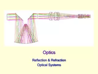
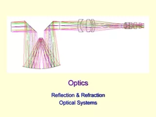
Optics Intro. Geometric Optics Raytracing. surface normal. same angle. Reflection. We describe the path of light as straight-line rays “geometrical optics” approach Reflection off a flat surface follows a simple rule: angle in (incidence) equals angle out

E N D
Optics Intro Geometric Optics Raytracing
UW ASTR 597 surface normal same angle Reflection • We describe the path of light as straight-line rays • “geometrical optics” approach • Reflection off a flat surface follows a simple rule: • angle in (incidence) equals angle out • angles measured from surface “normal” (perpendicular) exit ray incident ray
UW ASTR 597 A shortest path; equal angles B too long Reflection, continued • Also consistent with “principle of least time” • If going from point A to point B, reflecting off a mirror, the path traveled is also the most expedient (shortest) route
UW ASTR 597 “real” you “image” you Hall Mirror • Useful to think in terms of images mirror only needs to be half as high as you are tall. Your image will be twice as far from you as the mirror.
UW ASTR 597 Curved mirrors • What if the mirror isn’t flat? • light still follows the same rules, with local surface normal • Parabolic mirrors have exact focus • used in telescopes, backyard satellite dishes, etc. • also forms virtual image
UW ASTR 597 Refraction • Light also goes through some things • glass, water, eyeball, air • The presence of material slows light’s progress • interactions with electrical properties of atoms • The “light slowing factor” is called the index of refraction • glass has n = 1.52, meaning that light travels about 1.5 times slower in glass than in vacuum • water has n = 1.33 • air has n = 1.00028 • vacuum is n = 1.00000 (speed of light at full capacity)
UW ASTR 597 A Snell’s Law: n1sin1 = n2sin2 1 n1 = 1.0 n2 = 1.5 2 B Refraction at a plane surface • Light bends at interface between refractive indices • bends more the larger the difference in refractive index • can be effectively viewed as a “least time” behavior • get from A to B faster if you spend less time in the slow medium
UW ASTR 597 Driving Analogy • Let’s say your house is 12 furlongs off the road in the middle of a huge field of dirt • you can travel 5 furlongs per minute on the road, but only 3 furlongs per minute on the dirt • this means “refractive index” of the dirt is 5/3 = 1.667 • Starting from point A, you want to find the quickest route: • straight across (AD)—don’t mess with the road • right-angle turnoff (ACD)—stay on road as long as possible • angled turnoff (ABD)—compromise between the two A B C leg dist. t@5 t@3 AB 5 1 — AC 16 3.2 — AD 20 — 6.67 BD 15 — 5 CD 12 — 4 road dirt D (house) AD: 6.67 minutes ABD: 6.0 minutes: the optimal path is a “refracted” one ACD: 7.2 minutes Note: both right triangles in figure are 3-4-5
UW ASTR 597 n1 = 1.0 n2 = 1.5 Total Internal Reflection • At critical angle, refraction no longer occurs • thereafter, you get total internal reflection n2sin2 = n1sin1 crit = sin1(n1/n2) • for glass, the critical internal angle is 42° • for water, it’s 49° • a ray within the higher index medium cannot escape at shallower angles (look at sky from underwater…) incoming ray hugs surface 42°
UW ASTR 597 Refraction in Suburbia • Think of refraction as a pair of wheels on an axle going from sidewalk onto grass • wheel moves slower in grass, so the direction changes Note that the wheels move faster (bigger space) on the sidewalk, slower (closer) in the grass
UW ASTR 597 Even gets Total Internal Reflection Right • Moreover, this analogy is mathematically equivalent to the actual refraction phenomenon • can recover Snell’s law: n1sin1 = n2sin2 Wheel that hits sidewalk starts to go faster, which turns the axle, until the upper wheel re-enters the grass and goes straight again
UW ASTR 597 n1 = 1.5 n2 = 1.0 incoming ray (100%) 96% 4% 92% transmitted 0.16% 4% Reflections, Refractive offset • Let’s consider a thick piece of glass (n = 1.5), and the light paths associated with it • reflection fraction = [(n1– n2)/(n1 + n2)]2 • using n1 = 1.5, n2 = 1.0 (air), R = (0.5/2.5)2 = 0.04 = 4% image looks displaced due to jog 8% reflected in two reflections (front & back)
UW ASTR 597 Let’s get focused… • Just as with mirrors, curved lenses follow same rules as flat interfaces, using local surface normal A lens, with front and back curved surfaces, bends light twice, each diverting incoming ray towards centerline. Follows laws of refraction at each surface. Parallel rays, coming, for instance from a specific direction (like a distant bird) are focused by a convex (positive) lens to a focal point. Placing film at this point would record an image of the distant bird at a very specific spot on the film. Lenses map incoming angles into positions in the focal plane.
UW ASTR 597 pinhole object image at film plane object image at film plane lens Cameras, in brief In a pinhole camera, the hole is so small that light hitting any particular point on the film plane must have come from a particular direction outside the camera In a camera with a lens, the same applies: that a point on the film plane more-or-less corresponds to a direction outside the camera. Lenses have the important advantage of collecting more light than the pinhole admits
UW ASTR 597 Positive Lenses • Thicker in middle • Bend rays toward axis • Form real focus
UW ASTR 597 Negative Lenses • Thinner in middle • Bend rays away from the axis • Form virtual focus
UW ASTR 597 Raytracing made easier • In principle, to trace a ray, one must calculate the intersection of each ray with the complex lens surface, compute the surface normal here, then propagate to the next surface • computationally very cumbersome • We can make things easy on ourselves by making the following assumptions: • all rays are in the plane (2-d) • each lens is thin: height does not change across lens • each lens has a focal length (real or virtual) that is the same in both directions
UW ASTR 597 Thin Lens Benefits • If the lens is thin, we can say that a ray through the lens center is undeflected • real story not far from this, in fact: direction almost identical, just a jog • the jog gets smaller as the lens gets thinner
UW ASTR 597 Using the focus condition real foci virtual foci s = ∞ s’ = f s = ∞ s’ = f s = f s’ = ∞ s = f s’ = ∞ s = ∞ s’ = f s = ∞ s’ = f
UW ASTR 597 Tracing an arbitrary ray (positive lens) • draw an arbitrary ray toward lens • stop ray at middle of lens • note intersection of ray with focal plane • from intersection, draw guiding (helper) ray straight through center of lens (thus undeflected) • original ray leaves lens parallel to helper why?because parallel rays on one side of lens meet each other at the focal plane on the other side
UW ASTR 597 Tracing an arbitrary ray (negative lens) • draw an arbitrary ray toward lens • stop ray at middle of lens • draw helper ray through lens center (thus undeflected) parallel to the incident ray • note intersection of helper with focal plane • emerging ray will appear to come from this (virtual) focal point why?parallel rays into a negative lens appear to diverge from the same virtual focus on the input side
UW ASTR 597 Image Formation • Place arrow (object) on left, trace through image: • 1) along optical axis (no defl.); 2) parallel to axis, goes through far focus with optical axis ray; 3) through lens center; 4) through near-side focus, emerges parallel to optical axis; 5) arbitrary ray with helper • Note convergence at image position (smaller arrow) • could run backwards just as well
UW ASTR 597 Notes on Image Formation • Note the following: • image is inverted • image size proportional to the associated s-value: ray 3 proves it • both s and s’ are larger than f (s = 120; s’ = 80; f = 48) • Gaussian lens formula (simple form):
UW ASTR 597 Virtual Images • If the object is inside the focal length (s < f): • a virtual (and larger) image is formed • non-inverted • Ray numbers are same procedure as previous • This time s’ is negative: • s = 40; f = 60; s’ = 120 • negative image distances indicate virtual images
UW ASTR 597 The lens-maker’s formula • We saw the Gaussian lens formula before: • f is positive for positive lenses, negative for negative lenses • s is positive on left, s’ is positive on right • But in terms of the surface properties: • R1 is for the left surface (pos. if center of curvature to right) • R2 is for right surface (pos. if center of curvature to right) • bi-convex (as in prev. examples) has R1 > 0; R2 < 0 • n is the refractive index of the material (assume in air/vac)
UW ASTR 597 Deriving Gaussian Formula from Rays • Object has height, h; image height = h’ • tangent of ray 3 angle is h/s, so h’ = h(s’/s) • ray 2 angle is h/f, so h’ = (h/f)(s’ f) • set the two expressions for h’ equal, and divide by hs’ • the result will pop out • can do the same trick using virtual images too
UW ASTR 597 Lenses map directions into displacements • Two objects at infinity an angle apart produce distinct spots separated by • following geometry, = f·tan f· for small • hint: look at central rays • so lens turns angle () into displacement ()
UW ASTR 597 Telescope • A telescope has an “objective” lens and an eyepiece • sharing a focal plane; giving the eye the parallel light it wants • Everything goes as ratio of focal lengths: f1/f2 • magnification is just M = 2/1 = f1/f2 • after all: magnification is how much bigger things look • displacement at focal plane, = f11 = f22 relation above • ratio of collimated beam (pupil) sizes: P1/P2 = f1/f2 = M
UW ASTR 597 Reflector/Refractor Analogy • For the purposes of understanding a reflecting system, one may replace with lenses (which we know how to trace/analyze) • focal length and aperture the same; rays on other side • for a reflector, f = R/2 [compare to 1/f = (n 1)(1/R1 1/R2) for lens] • for n = 1.5, R2 = R1 (symmetric lens), f = R • so glass lens needs twice the curvature of a mirror
UW ASTR 597 Parabolic Example Take the parabola: y = x2 Slope is y’ = 2x Curvature is y’’ = 2 So R = 1/y’’ = 0.5 Slope is 1 (45) at: x = 0.5; y = 0.25 So focus is at 0.25: f = R/2 Note that pathlength to focus is the same for depicted ray and one along x = 0
UW ASTR 597 Cassegrain Telescope • A Cassegrain telescope can be modeled as as positive and negative lens • eyepiece not shown: only up to focus • Final focus depends on placement of negative lens • if |s| = |f2|, light is collimated; if |s| > |f2|, light will diverge • both s and f2 are negative • For the Apache Point 3.5 meter telescope, for example: • f1 = 6.12 m; f2 = 1.60 m; d12 = 4.8 m; s = d12 f1 = 1.32 m • yields s’ = 7.5 m using 1/s + 1/s’ = 1/f2
UW ASTR 597 Cassegrain focus • Abstracting mirrors as lenses, then lenses as sticks: • trace central ray with angle 1 • figure out 2 and then focal length given s’ and d12 • y2 = d121 (adopt convention where 1 is negative as drawn) • y1 = f21 (f2 is negative: negative lens) • 2 = (y1 y2)/f2 = 1(f2 d12)/f2 • yf = y2 + 2s’ = 1(d12 + s’(f2 d12)/f2) • feff = d12 + s’(f2 d12)/f2 = f1s’/s after lots of algebra • for Apache Point 3.5 meter, this comes out to 35 meters
UW ASTR 597 f-numbers f = D f = 4D • The f-number is a useful characteristic of a lens or system of lenses/mirrors • Simply = f/D • where f is the focal length, and D is the aperture (diameter) • “fast” converging beams (low f-number) are optically demanding to make without aberrations • “slow” converging beams (large f-number) are easier to make • aberrations are proportional to 1/2 • so pay the price for going “fast” D D f/4 beam: “slow” f/1 beam: “fast”
UW ASTR 597 f-numbers, compared • Lens curvature to scale for n = 1.5 • obviously slow lenses are easier to fabricate: less curvature
UW ASTR 597 Pupils • Consider two “field points” on the focal plane • e.g., two stars some angle apart • The rays obviously all overlap at the aperture • called the entrance pupil • The rays are separate at the focus (completely distinct) • Then overlap again at exit pupil, behind eyepiece • want your pupil here • just an image of the entrance pupil satisfying 1/s’ + 1/(f1 + f2) = 1/f2 • size is smaller than entrance pupil by magnification factor • M = f1/f2; in this picture, f1 = 48; f2 = 12; M = 4; s’ = 15
UW ASTR 597 Pupils within Pupils • Looking at three stars (red, green, blue) through telescope, eye position is important • So is pupil size compared to eye pupil • dark adapted pupil up to 7 mm diameter (2–3 mm in daylight) • sets limit on minimum magnification (if you want to use the full aperture) • 210 mm aperture telescope must have M > 30 • for f/5 scope, means f2 < 35 mm; f/10 scope means f2 < 70 mm • 3.5-m scope means M > 500; at f/10, f2 < 70 mm
UW ASTR 597 Vignetting • Rays that don’t make it through an optical system are said to be vignetted (shadowed) • maybe a lens isn’t big enough • maybe your eye’s pupil isn’t big enough, or is improperly placed • Often appears as a gradual darkening as a function of distance from the field center • the farther out you go, the bigger your lenses need to be • every optical system has a limited (unvignetted) field of view • beyond this, throughput goes down
UW ASTR 597 Infrared Cold Stop • An infrared detector is very sensitive to terrestrial heat • so want to keep off of detector • if detector located at primary focal plane, it is inundated with emission from surroundings and telescope structure • note black lines intersecting primary focal plane • Putting a “cold” stop at a pupil plane eliminates stray emission • cool to LN2; image of primary objective onto cold stop • only light from the primary passes through; detector focal plane then limits field of view to interesting bit • Also the right place for filters, who prefer collimated light
UW ASTR 597 Raytrace Simulations • In Google, type in: phet • top link is one to University of Colorado physics education page • on this page, click: go to simulations • on the left-hand bar, go to: light and radiation • then click the geometric optics simulation link (picture) • Can play with lots of parameters • real and virtual images • lens radius of curvature, diameter, and refractive index • see principle rays (ones you’d use to raytrace) • see marginal rays • use a light source and screen • see the effect of two sources
UW ASTR 597 Aberrations: the real world • Lenses are thick, sin • sin 3/6 + 5/120 7/5040 + … • tan + 3/3 + 25/15 + 177/315 + … • Different types of aberration (imperfection) • spherical aberration • all spherical lenses possess; parabolic reflector does not • coma • off-axis ailment: even aspheric elements have this • chromatic aberration • in refractive systems only: refractive index is function of • astigmatism • if on axis, then lens asymmetry; but can arise off-axis in any system • field curvature/distortion • detectors are flat: want to eliminate significant field curvature
UW ASTR 597 Spherical Aberration • Rays at different heights focus at different points • Makes for a mushy focus, with a halo • Positive spherical lenses have positive S.A., where exterior rays focus closer to lens • Negative lenses have negative S.A., as do plates of glass in a converging beam • “Overcorrecting” a positive lens (going too far in making asphere) results in neg. S.A. neg. S.A. lens side zero S.A. pos. S.A.
UW ASTR 597 Coma • Off-axis rays meet at different places depending on ray height • Leads to asymmetric image, looking something like a comet (with nucleus and flared tail) • thus the name coma • As with all aberrations, gets worse with “faster” lenses • Exists in parabolic reflectors, even if no spherical aberration
UW ASTR 597 Chromatic Aberration • Glass has slightly different refractive index as a function of wavelength • so not all colors will come to focus at the same place • leads to colored blur • why a prism works • Fixed by pairing glasses with different dispersions (dn/d) • typically a positive lens of one flavor paired with a negative lens of the other • can get cancellation of aberration • also helps spherical aberration to have multiple surfaces (more design freedom)
UW ASTR 597 Zemax Examples
UW ASTR 597 Raytracing Program • While it may not be Zemax, I’ve cobbled together a C-program (and Python) to do raytracing of any number of lenses/mirrors • restricted to the following conditions: • ray path is sequential: hitting surfaces in order defined • elements are flat or have conic surfaces • refractive index is constant, and ignorant of dispersion • 2-d only (though later will migrate to 3-d) • We can use this package to: • analyze simple lens configurations • look at aberrations • build lens systems (beam expanders, telescopes)
UW ASTR 597 Raytracing Algorithm • Detailed math available on website (raytrace link) • Basically, compute intersection of ray with surface, then apply Snell’s Law • Can have as many surfaces as you want! • Must take care in defining physical systems • e.g., make sure lens is thick enough for the diameter you need
UW ASTR 597 Representing Mirrors • The default/conventional behavior has light going from left to right (toward positive z) • But changing the sign of the refractive index signals a change of direction • after all, refractive index indicates the speed of light in a medium, and the speed changes sign at a reflection • Example: APO 3.5 m scope (dims in mm) 2 1.0 -1.0 0.0 -12279.7 -1.01927 1.0 -4833.421 -3164.172 -2.18427 • Note index changes from +1.0 initially to -1.0, then back to +1.0