Download
1 / 56
620 likes | 1.29k Views
Course Outline (Tentative). Fundamental Concepts of Signals and Systems Signals Systems Linear Time-Invariant (LTI) Systems Convolution integral and sum Properties of LTI Systems … Fourier Series Response to complex exponentials Harmonically related complex exponentials …

E N D
Course Outline (Tentative) • Fundamental Concepts of Signals and Systems • Signals • Systems • Linear Time-Invariant (LTI) Systems • Convolution integral and sum • Properties of LTI Systems … • Fourier Series • Response to complex exponentials • Harmonically related complex exponentials … • Fourier Integral • Fourier Transform & Properties … • Modulation (An application example) • Discrete-Time Frequency Domain Methods • DT Fourier Series • DT Fourier Transform • Sampling Theorem • Z Transform • Laplace Transform
+ RC circuit - What is Signal? • Signal is the variation of a physical phenomenon /quantity with respect to one or more independent variable • A signal is a function. Example 1: Voltage on a capacitor as a function of time.
Index S S F M W T T Fig. Stock exchange What is Signal? Example 3:Image as a function of x-y coordinates (e.g. 256 X 256 pixel image) Example 2 : Closing value of the stock exchange indexas a function of days
Continuous-Time vs. Discrete Time • Signals are classified as continuous-time (CT) signals and discrete-time (DT) signals based on the continuity of the independent variable! • In CT signals, the independent variable is continuous (See Example 1 (Time)) • In DT signals, the independent variable is discrete (See Ex 2 (Days), Example 3 (x-y coordinates, also a 2-D signal)) • DT signal is defined only for specified time instants! • also referred as DT sequence!
Continuous-Time vs. Discrete Time • The postfix (-time) is accepted as a convention, although some independent variables are not time • To distinguish CT and DT signals, t is used to denote CT independent variable in (.), and n is used to denote DT independent variable in [.] • Discrete x[n], n is integer • Continuous x(t), t is real • Signals can be represented in mathematical form: • x(t) = et, x[n] = n/2 • y(t) = • Discrete signals can also be represented as sequences: • {y[n]} = {…,1,0,1,0,1,0,1,0,1,0,…}
... ... ... ... 1 -3 -2 -1 0 2 3 4 0 (Fig.1.7 Oppenheim) Continuous-Time vs. Discrete-Time Graphically, • It is meaningless to say 3/2th sample of a DT signal because it is not defined. • The signal values may well also be complex numbers (e.g. Phasor of the capacitor voltage in Example 1 when the input is sinusoidal and R is time varying)
Signal Energy and Power • In many applications, signals are directly related to physical quantities capturing power and energy in physical systems • Total energy of a CT signal over is • The time average of total energy is and referred to as average power of over • Similarly, total energy of a DT signal over is • Average power of over is
Note: Signals with have Signal Energy and Power • For infinite time intervals: • Energy: accumulation of absolute of the signal • Signals with are of finite energy • In order to define the power over infinite intervals we need to take limit of the average: Total energy in CT signal Total energy in DT signal
Signal Energy and Power • Energysignal iff 0<E<, and so P=0 • e.g: • Power signal iff 0<P<, and so E= • e.g: • Neither energy nor power, when both E and P are infinite • e.g: • .
Transformation of Independent Variable • Sometimes we need to change the independent variable axis for theoretical analysis or for just practical purposes (both in CT and DT signals) • Time shift • Time reversal • Time scaling (reverse playing of magnetic tape) (slow playing, fast playing)
Examples of Transformations x[n] Time shift If n0 > 0 x[n-n0] is the delayed version of x[n] (Each point in x[n] occurs later in x[n-n0]) . . . . . . n x[n-n0] . . . . . . . . . . . n n0
Examples of Transformations x(t) Time shift t0 < 0 x(t-t0) is an advanced version of x(t) t x(t-t0) t t0
Examples of Transformations x(t) Reflection about t=0 Time reversal t x(-t) t
x(2t) t x(t/2) t Examples of Transformations Time scaling x(t) t compressed! stretched!
x(t) 1 t 1 2 0 x(t+1) 1 (It is a time shift to the left) t 0 -1 1 x(-t+1) 1 (Time reversal of x(t+1)) t 0 -1 1 Examples of Transformations • It is possible to transform the independent variable with a general nonlinear function h(t) ( we can find x(h(t)) ) • However, we are interested in 1st order polynomial transforms of t, i.e., x(at+b) Given the signal x(t): Let us find x(t+1): Let us find x(-t+1):
x(t+1) 1 t 0 -1 1 x((3/2)t+1) 1 t 2/3 -2/3 0 Examples of Transformations • For the general case, i.e., x(at+b), • first apply the shift (b), • and then perform time scaling (or reversal) based on a. Example: Find x(3t/2+1)
Periodic Signals • A periodic signal satisfies: Example: A CT periodic signal • If x(t)is periodic with T then • Thus, x(t)is also periodic with 2T, 3T, 4T, ... • The fundamental periodT0 of x(t)is the smallest valueof T for which holds
Periodic Signals • A non-periodic signal is called aperiodic. • For DT we must have Here the smallest N can be 1, • The smallest positive value N0 of N is the fundamental period Period must beinteger! a constant signal
x(t) odd x(t) even t t Even and Odd Signals • If even signal (symmetric wrt y-axis) • If odd signal (symmetric wrt origin) • Decomposition of signals to even and odd parts:
a > 0 a < 0 x(t) x(t) C C t t Exponential and Sinusoidal Signals • Occur frequently and serve as building blocks to construct many other signals • CT Complex Exponential: where a and C are in general complex. • Depending on the values of these parameters, the complex exponential can exhibit several different characteristics Real Exponential (C and a are real)
for periodicity = 1 Exponential and Sinusoidal Signals • Periodic Complex Exponential (Creal, a purely imaginary) • Is this function periodic? • The fundamental period is • Thus, the signals ejω0tand e-jω0thave the same fundamental period
Exponential and Sinusoidal Signals • Using the Euler’s relations: and by substituting, we can express: Sinusoidals in terms of complex exponentials
Exponential and Sinusoidal Signals Alternatively, CT sinusoidal signal
Exponential and Sinusoidal Signals • Complex periodic exponential and sinusoidal signals are of infinite total energy but finite average power • As the upper limit of integrand is increased as • However, always • Thus, Finite average power!
Harmonically Related Complex Exponentials • Set of periodic exponentials with fundamental frequencies that are multiplies of a single positive frequency • kthharmonicxk(t) is still periodic with T0 as well • Harmonic (from music): tones resulting from variations in acoustic pressures that are integer multiples of a fundamental frequency • Used to build very rich class of periodic signals
envelope General Complex Exponential Signals Here, C and a are general complex numbers Say, (Real and imaginary parts) Growing and damping sinusoids for r>0 and r<0
DT Sinusoidal Signals Infinite energy, finite average power with 1. General complex exp signals
Periodicity Properties of DT Signals • So the signal with freq 0 is the same as the signal with 0+2 • This is very different from CT complex exponentials • CT exponentials has distinct frequency values 0+2k, k Z Result: It is sufficient to consider an interval from 0 to 0+2 to completely characterize the DT complex exponential!
Periodicity Properties of DT Signals What about the periodicity of DT complex exponentials?
Periodicity Properties of DT SignalsExamples • OBSERVATION: • With no common factors between N and m, N in (***) is the fundamental period of the signal • Hence, if we take common factors out • Comparison of Periodicity of CT and DT Signals: • Consider x(t) and x[n] x(t) is periodic with T=12, x[n] is periodic with N=12.
Periodicity Properties of DT SignalsExamples • if andx(t) is periodic with 31/4. • In DT there can be no fractional periods, for x[n] we have then N=31. If and x(t) is periodic with 12, but x[n] is not periodic, because there is no way to express it as in (***) .
Harmonically Related Complex Exponentials(Discrete Time) • Set of periodic exponentials with a common period N • Signals at frequencies multiples of (from 0N=2m) • In CT, all of the HRCE, are distinct • Different in DT case!
Harmonically Related Complex Exponentials(Discrete Time) • Let’s look at (k+N)th harmonic: • Only N distinct periodic exponentials in k[n] !! • That is,
δ[n] - - - - - - n u[n] - - - - - - Unit Impulse and Unit Step Functions • Basic signals used to construct and represent other signals DT unit impulse: DT unit step: Relation between DT unit impulse and unit step (?): Unit impulse (unit sample) n (DT unit impulse is the first difference of the DT step)
Interval of summation [n-k] - - - - - - k n 0 Interval of summation [n-k] n<0 n>0 - - - - - - k n 0 Sampling property Unit Impulse and Unit Step Functions (DT step is the running sum of DT unit sample) More generally for a unit impulse [n-n0] at n0 :
u(t) t 1 t 0 Unit Impulse and Unit Step Functions (Continuous-Time) CT unit step: CT impulse: δ(t) CT unit impulse is the 1st derivative of the unit sample CT unit step is the running integral of the unit impulse
1 t 0 1/ 1 t t 0 0 Continuous-Time Impulse • CT impulse is the 1st derivative of unit step • There is discontinuity at t=0, therefore we define as
Continuous-Time Impulse REMARKS: • Signal of a unit area • Derivative of unit step function • Sampling property • The integral of product of (t) and (t) equals (0) for any (t) continuous at the origin and if the interval of integration includes the origin, i.e.,
x[n] y[n] DT System x(t) y(t) CT System CT and DT SystemsWhat is a system? • A system: any process that results in the transformation of signals • A system has an input-output relationship • Discrete-Time System:x[n] y[n] :y[n] = H[x[n]] • Continuous -Time System:x(t) y(t) :y(t) = H(x(t))
+ RC circuit - CT and DT SystemsExamples • In CT, differential equations are examples of systems • Zero state response of the capacitor voltage in a series RC circuit • In DT, we have difference equations • Consider a bank account with %1 monthly interest rate added on: vc(t): output, vs(t): input y[n]: output: account balance at the end of each month x[n]: input: net deposit (deposits-withdrawals)
x(t) y(t) System 1 H1 System 2 H2 System 1 H1 y(t) x(t) + System 1 H2 Interconnection of Systems • Series (or cascade) Connection:y(t) = H2( H1( x(t) ) ) • e.g. radio receiver followed by an amplifier • Parallel Connection:y(t) = H2( x(t) ) + H1( x(t) ) • e.g. phone line connecting parallel phone microphones
x(t) y(t) System 1 H1 + System 2 H2 Interconnection of Systems • Previous interconnections were “feedforward systems” • The systems has no idea what the output is • Feedback Connection:y(t) = H2( y(t) ) + H1( x(t) ) • In feedback connection, the system has the knowledge of output • e.g. cruise control • Possible to have combinations of connections..
System PropertiesMemory vs. Memoryless Systems • Memoryless Systems: System output y(t) depends only on the input at time t, i.e. y(t) is a function of x(t). • e.g. y(t)=2x(t) • Memory Systems: System output y(t) depends on input at past or future of the current time t, i.e. y(t) is a function of x() where - < <. • Examples: • A resistor: y(t) = R x(t) • A capacitor: • A one unit delayer: y[n] = x[n-1] • An accumulator:
x(t) y(t) w(t)=x(t) System Inverse System Not invertible System PropertiesInvertibility • A system is invertible if distinct inputs result in distinct outputs. • If a system is invertible, then there exists an inverse system which converts output of the original system to the original input. • Examples:
Non-causal Non-causal Causal System PropertiesCausality • A system is causal if the output at any time depends only on values of the input at the present time and in the past • Examples: • Capacitor voltage in series RC circuit (casual) • Systems of practical importance are usually casual • However, with pre-recorded data available we do not constrain ourselves to causal systems (or if independent variable is not time, any example??) (For n<0, system requires future inputs) Averaging system in a block of data