Log-linear Approximate Present Value Models: Empirical Finance Insights
Dive into the sources impacting stock prices over time, quantify their influence, and assess their persistence using log-linear models and approximations. Explore the relationship between stock prices, dividends, and yields based on key financial theories. Implement empirical approaches, including vector autoregression (VAR) methods, to analyze the intertemporal and cross-sectional behavior of expected returns. Delve into Equity Return Volatility analysis, assessing the role of shock persistence and robust estimations. Investigate diverse models of expected returns, testing theories against real-world financial data from influential scholars like J. Campbell and R. Shiller.

Log-linear Approximate Present Value Models: Empirical Finance Insights
E N D
Presentation Transcript
Log-linear approximate present-value models FINA790C Empirical Finance HKUST Spring 2006
Motivation • What are the sources of changes in stock prices over time? • Can we quantify their impact? • How persistent is their impact? • Background: J. Campbell and R. Shiller, “The dividend-price ratio and expectations of future dividends and discount factors” RFS 1(3), Fall 1988; J. Campbell and R. Shiller, “Stock prices, earnings and expected dividends” JF 43(3), July 1988.
Stock prices and dividend yields • To study these issues we need to be able to relate prices to underlying “fundamentals” • ln(Rt+1) = ln(Pt+1 + Dt+1) – ln(Pt) = ln(Pt+1) – ln(Pt) + ln( 1 + DYt+1) • Or rt+1 = pt+1 + ln( 1 + exp(t+1) ) - pt where t+1 = ln(DYt+1) and DYt+1 is the dividend yield at t+1
Returns, prices and yields: an approximate relation • Suppose t is a stationary stochastic process with a constant mean. Then we can expand f() = ln(1+exp()) in a Taylor series around its mean (call it * = d* - p*) • This gives rt+1≈ k + pt+1 + (1- )dt+1 – pt where k = -ln()-(1- )ln( (1/ )-1 ) and = 1/(1+exp(*))
Static, constant growth case • Suppose dividend growth is constant and return is constant: Dt+1/Dt = exp(g) = Pt+1/Pt , (Pt+1+Dt+1)/Pt = exp(r) • Note exp(g-r) = Pt+1/(Pt+1+Dt+1) constantand (1/exp(g-r))-1 = Dt+1/Pt+1 so DY is constant • Since k + pt+1 + (1- )dt+1 – pt = k + (1- )(dt+1 – pt+1)+ pt+1– pt in this case the approximation is exact
Discounting formula • Or pt = k + pt+1 + (1- )dt+1 – rt Recursively substitute for pt+1 to get pt = k(1++2+… + (1- )dt+1 + (1- )dt+2 + 2(1- )dt+3 + … - rt+1 - rt+2 - 2rt+3 - … • Or pt = {k/(1- )} + j{(1- )dt+1+j - rt+1+j} (assuming lim jpt+j = 0 as j →∞)
Loglinear approximate present value relation • Take conditional expectations pt = {k/(1- )} + Etj{(1- )dt+1+j - rt+1+j} • The log dividend-price ratio t = -{k/(1- )} + Etj{-Δdt+1+j + rt+1+j}
What moves stock prices? • Unexpected stock returns are given by rt+1 - Etrt+1 = (Et+1 - Et) jΔdt+1+j - (Et+1 - Et) jrt+1+j • Or rt+1 = dt+1 - rt+1
Example • Suppose expected returns are given by Etrt+1 = r* + xt where xt is an observable zero mean variable that follows an AR(1) process xt+1 = xt + ut+1 (-1≤ ≤+1) • In this case rt+1 = ut+1/(1- ) • The importance of movements in expected returns for stock price volatility is var(rt+1)/var(rt+1) = (1-2)(/(1-))2(R2/(1-R2)) where R2 is the fraction of the variance of return that is predictable
Excess returns • If the log riskfree rate is rft+1 then excess log returns are et+1 = rt+1 - rft+1 • Substituting for rt+1 gives et+1 - Etet+1 = (Et+1 - Et) jΔdt+1+j - (Et+1 - Et) jrft+1+j - (Et+1 - Et) jet+1+j or et+1 = dt+1 - ft+1 - et+1
Empirical implementation • Vector autoregression (VAR) approach • Description and variance decompositions • Testing models for intertemporal behavior of expected returns • Testing models for cross-sectional behavior of expected returns (see J. Campbell (1996),”Understanding risk and return”, Journal of Political Economy 104(2), April, 298-345)
VAR approach • Define k-element vector zt+1 that includes as its first element rt+1. The other variables are potential predictors of returns (such as t+1, Δdt+1 ). • Estimate a vector autoregression for zt+1 as follows zt+1 = Azt + wt+1 • Note that Etzt+k = Akzt and in particular Etrt+1+j = e1’Aj+1zt where e1 is k-element vector with first element 1 and others 0.
Return variance decomposition • So rt+1 = (Et+1 - Et) jrt+1+j = e1’ jAjwt+1 =e1’A(I - A)-1wt+1 = ’wt+1 • Since rt+1 - Etrt+1 = rt+1 = e1’ wt+1 = dt+1 - rt+1 this gives dt+1 = (e1’ + ’)wt+1
Persistence measure • How long do shocks to expected returns persist? Shock to one-period ahead expected return = (Et+1 - Et)rt+2 = ut+1 = e1’Awt+1 • Define Pr = σ(rt+1)/ σ(ut+1) = σ(’wt+1)/ σ(e1’Awt+1)
Estimation • Estimate • VAR coefficients A • Variance matrix of innovations var(wt+1) • Calculate (nonlinear) functions of A and estimate standard errors by delta method
Testing expected return models • Suppose we have a theory that specifies the time series behavior of Etrt+1 = Ett+1 • For example • Etrt+1 = constant • Etrt+1 = EtΔlnCt+1 • Etrt+1 = Etrt+12 • We can see what this implies for the behavior of the VAR
Example: Constant expected return • If expected returns are constant then the log dividend yield is t = -{k/(1- )} + Etj{-Δdt+1+j + } = (-k)/(1- )} + Etj{-Δdt+1+j} • If zt = [t–Δdt … ]’ then e1’zt = e2’Azt + e2’A2zt + e2’2A3zt … = e2’A(I - A)-1zt • To hold for all zt we must have e1’= e2’A(I - A)-1