Distribution Ray Tracing
Distribution Ray Tracing. Reading. Required: Watt, sections 10.6 ,14.8. Further reading: A. Glassner. An Introduction to Ray Tracing. Academic Press, 1989. [In the lab.]

Distribution Ray Tracing
E N D
Presentation Transcript
Reading • Required: • Watt, sections 10.6 ,14.8. • Further reading: • A. Glassner. An Introduction to Ray Tracing. Academic Press, 1989. [In the lab.] • Robert L. Cook, Thomas Porter, Loren Carpenter.“Distributed Ray Tracing.” Computer Graphics (Proceedings of SIGGRAPH 84). 18 (3). pp. 137-145. 1984. • James T. Kajiya. “The Rendering Equation.” Computer Graphics (Proceedings of SIGGRAPH 86). 20 (4). pp. 143-150. 1986. • Henrik Wann Jensen, “Basic Monte Carlo Integration”, Appendix A from book “Realistic Image Synthesis Using Photon Mapping”. University of Texas at Austin CS384G - Computer Graphics Fall 2008 Don Fussell 2
Pixel anti-aliasing No anti-aliasing Pixel anti-aliasing University of Texas at Austin CS384G - Computer Graphics Fall 2008 Don Fussell 3
Surface reflection equation • In reality, surfaces do not reflect in a mirror-like fashion. • To compute the reflection from a real surface, we would actually need to solve the surface reflection equation: • How might we represent light from a single direction? • We can plot the reflected light as a function of viewing angle for multiple light source contributions: University of Texas at Austin CS384G - Computer Graphics Fall 2008 Don Fussell 4
Simulating gloss and translucency • The mirror-like form of reflection, when used to approximate glossy surfaces, introduces a kind of aliasing, because we are undersampling reflection (and refraction). • For example: • Distributing rays over reflection directions gives: University of Texas at Austin CS384G - Computer Graphics Fall 2008 Don Fussell 5
Reflection anti-aliasing Reflection anti-aliasing University of Texas at Austin CS384G - Computer Graphics Fall 2008 Don Fussell 6
Full anti-aliasing Full anti-aliasing…lots of nested integrals! Computing these integrals is prohibitively expensive. We’ll look at ways to approximate integrals… University of Texas at Austin CS384G - Computer Graphics Fall 2008 Don Fussell 7
Approximating integrals • Let’s say we want to compute the integral of a function: • If f(x) is not known analytically, but can be evaluated, then we can approximate the integral by: • Evaluating an integral in this manner is called quadrature. University of Texas at Austin CS384G - Computer Graphics Fall 2008 Don Fussell 8
Integrals as expected values • An alternative to distributing the sample positions regularly is to distribute them stochastically. • Let’s say the position in x is a random variable X, which is distributed according to p(x), a probability density function (strictly positive that integrates to unity). • Now let’s consider a function of that random variable, f(X)/p(X). What is the expected value of this new random variable? • First, recall the expected value of a function g(X): • Then, the expected value of f(X)/p(X) is: University of Texas at Austin CS384G - Computer Graphics Fall 2008 Don Fussell 9
Monte Carlo integration • Thus, given a set of samples positions, Xi, we can estimate the integral as: • This procedure is known as Monte Carlo integration. • The trick is getting as accurate as possible with as few samples as possible. • More concretely, we would like the variance of the estimate of the integral to be low: • The name of the game is variance reduction… University of Texas at Austin CS384G - Computer Graphics Fall 2008 Don Fussell 10
Uniform sampling • One approach is uniform sampling (i.e., choosing X from a uniform distribution): University of Texas at Austin CS384G - Computer Graphics Fall 2008 Don Fussell 11
Importance sampling • A better approach, if f(x) is positive, would be to choose p(x) ~ f(x). In fact, this choice would be optimal. • Why don’t we just do that? • Alternatively, we can use heuristics to guess where f(x) will be large. This approach is called importance sampling. University of Texas at Austin CS384G - Computer Graphics Fall 2008 Don Fussell 12
Summing over ray paths We can think of this problem in terms of enumerated rays: The intensity at a pixel is the sum over the primary rays: For a given primary ray, its intensity depends on secondary rays: Substituting back in: University of Texas at Austin CS384G - Computer Graphics Fall 2008 Don Fussell 13
Summing over ray paths We can incorporate tertiary rays next: Each triple i,j,k corresponds to a ray path: So, we can see that ray tracing is a way to approximate a complex, nested light transport integral with a summation over ray paths (of arbitrary length!). Problem: too expensive to sum over all paths. Solution: choose a small number of “good” paths. University of Texas at Austin CS384G - Computer Graphics Fall 2008 Don Fussell 14
Whitted integration • An anti-aliased Whitted ray tracer chooses very specific paths, i.e., paths starting on a regular sub-pixel grid with only perfect reflections (and refractions) that terminate at the light source. • One problem with this approach is that it doesn’t account for non-mirror reflection at surfaces. University of Texas at Austin CS384G - Computer Graphics Fall 2008 Don Fussell 15
Monte Carlo path tracing • Instead, we could choose paths starting from random sub-pixel locations with completely random decisions about reflection (and refraction). This approach is called Monte Carlo path tracing [Kajiya86]. • The advantage of this approach is that the answer is known to be unbiased and will converge to the right answer. University of Texas at Austin CS384G - Computer Graphics Fall 2008 Don Fussell 16
Importance sampling • The disadvantage of the completely random generation of rays is the fact that it samples unimportant paths and neglects important ones. • This means that you need a lot of rays to converge to a good answer. • The solution is to re-inject Whitted-like ideas: spawn rays to the light, and spawn rays that favor the specular direction. University of Texas at Austin CS384G - Computer Graphics Fall 2008 Don Fussell 17
Stratified sampling • Another method that gives faster convergence is stratified sampling. • E.g., for sub-pixel samples: • We call this a jittered sampling pattern. • One interesting side effect of these stochastic sampling patterns is that they actually injects noise into the solution (slightly grainier images). This noise tends to be less objectionable than aliasing artifacts. University of Texas at Austin CS384G - Computer Graphics Fall 2008 Don Fussell 18
Distribution ray tracing • These ideas can be combined to give a particular method called distribution ray tracing [Cook84]: • uses non-uniform (jittered) samples. • replaces aliasing artifacts with noise. • provides additional effects by distributing rays to sample: • Reflections and refractions • Light source area • Camera lens area • Time • [Originally called “distributed ray tracing,” but we will call it distribution ray tracing so as not to confuse with parallel computing.] University of Texas at Austin CS384G - Computer Graphics Fall 2008 Don Fussell 19
DRT pseudocode • TraceImage() looks basically the same, except now each pixel records the average color of jittered sub-pixel rays. functiontraceImage (scene): for each pixel (i, j) in image do I(i, j) 0 for each sub-pixel id in (i,j) do s pixelToWorld(jitter(i, j, id)) pCOP d(s - p).normalize() I(i, j) I(i, j) + traceRay(scene, p, d, id) end for I(i, j) I(i, j)/numSubPixels end for end function • A typical choice is numSubPixels = 4*4. University of Texas at Austin CS384G - Computer Graphics Fall 2008 Don Fussell 20
DRT pseudocode (cont’d) • Now consider traceRay(), modified to handle (only) opaque glossy surfaces: functiontraceRay(scene, p, d, id): (q, N, material) intersect (scene, p, d) I shade(…) R jitteredReflectDirection(N, -d, id) I I + material.kr traceRay(scene, q, R, id) return I end function University of Texas at Austin CS384G - Computer Graphics Fall 2008 Don Fussell 21
Pre-sampling glossy reflections University of Texas at Austin CS384G - Computer Graphics Fall 2008 Don Fussell 22
Soft shadows • Distributing rays over light source area gives: University of Texas at Austin CS384G - Computer Graphics Fall 2008 Don Fussell 23
The pinhole camera • The first camera - “camera obscura” - known to Aristotle. • In 3D, we can visualize the blur induced by the pinhole (a.k.a., aperture): • Q: How would we reduce blur? University of Texas at Austin CS384G - Computer Graphics Fall 2008 Don Fussell 24
Shrinking the pinhole • Q: How can we simulate a pinhole camera more accurately? • Q: What happens as we continue to shrink the aperture? University of Texas at Austin CS384G - Computer Graphics Fall 2008 Don Fussell 25
Shrinking the pinhole, cont’d University of Texas at Austin CS384G - Computer Graphics Fall 2008 Don Fussell 26
Lenses Pinhole cameras in the real world require small apertures to keep the image in focus. Lenses focus a bundle of rays to one point => can have larger aperture. For a “thin” lens, we can approximately calculate where an object point will be in focus using the the Gaussian lens formula: where f is the focal length of the lens. University of Texas at Austin CS384G - Computer Graphics Fall 2008 Don Fussell 27
Depth of field • Lenses do have some limitations. • The most noticeable is the fact that points that are not in the object plane will appear out of focus. • The depth of field is a measure of how far from the object plane points can be before appearing “too blurry. University of Texas at Austin CS384G - Computer Graphics Fall 2008 Don Fussell 28
Simulating depth of field • Distributing rays over a finite aperture gives: University of Texas at Austin CS384G - Computer Graphics Fall 2008 Don Fussell 29
Chaining the ray id’s • In general, you can trace rays through a scene and keep track of their id’s to handle all of these effects: University of Texas at Austin CS384G - Computer Graphics Fall 2008 Don Fussell 30
DRT to simulate motion blur • Distributing rays over time gives: University of Texas at Austin CS384G - Computer Graphics Fall 2008 Don Fussell 31