Download
1 / 44
460 likes | 589 Views
Chapter 8 - Processes. Scheduling models: FCFS - First Come First Serve ; aka FIFO - First In First Out; considered fair scheduling. Figure 8.1: supermarket scheduling

E N D
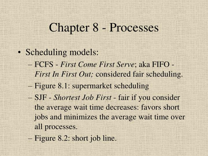
Chapter 8 - Processes • Scheduling models: • FCFS - First Come First Serve; aka FIFO - First In First Out; considered fair scheduling. • Figure 8.1: supermarket scheduling • SJF - Shortest Job First - fair if you consider the average wait time decreases: favors short jobs and minimizes the average wait time over all processes. • Figure 8.2: short job line.
Scheduling: • Highest-Response-Ratio-Next: discriminates less against long jobs (copy room analogy) • HRRN: • response ratio = (wait time + job time) / job time • Pick job with highest response ratio to go next. • The longer you wait, the better chance you get to go next. • Priority scheduling: Do the task with the highest priority first (or next). Difficult part is determining the priority values. • Deadline scheduling: Run the one that has to finish the soonest.
Scheduling: • Round Robin - Take turns with the resource; 10-minute video game analogy (Figure 8.3). • Round Robin lends itself well to preempted resources. • Round Robin scheduling of processes in an operating system is preferred, since preemption of the CPU is relatively cheap. • Preemptive Scheduling Methods • All follow the classic process flow diagram (Figure 8.4) with a timer enforcing preemption. • The Dispatcher() selects a new candidate from the ready queue; we are interested in the selection method.
Preemptive Round-Robin Scheduling • Pick first process in ready queue. • Set the timer to the time quantum or time slice value and let the process run. • When timer expires, put this process at the end of the list and pick the next process in the ready queue, assigning it a time quantum, etc. • Must select a reasonable size for the time slice. • One model: • Include context switch overhead in time slice • Suppose context switch time was 200 microsecs • Can measure the time slice in units of context switch times; 10 milliseconds = 50 context switches = 10,000 microsecs
Preemptive Round-Robin Scheduling • One model (continued): • If time slice = 1 context switch time, overhead for context switching is 100 percent. • If time slice = 100 context switch times, overhead for context switch is 1 percent. • In general, this is 1/N percent overhead; Figure 8.5 shows the curve. • End result: bad to have a very small time slice; bad to have a very long time slice (if interactive response is important). • Could pick a target interactive response of, say, 1/4 of a second and set the time slice to 250 milliseconds/NumberOfProcesses.
Preemptive Round-Robin Scheduling • Under large ready queue sizes, round robin degrades interactive response time, since the wait time is a function of the size of the queue. • Can adjust the time quantum based on the size of the ready queue (adaptive RR). • Multi-level queues • To alleviate this, the process scheduling algorithm can create a multi-tiered queuing system. • 2 queue example: any jobs (processes) in the top queue get scheduled before any in the bottom queue. A process that uses up it’s entire time slice is moved into the bottom queue (Figure 8.6).
Multi-level queues • Can extend to 3 queues that have variable parameters determining the job flow between the queues (Figure 8.7). • Dispatcher will select a job in Queue 1, else Queue 2 else finally Queue 3. • Let q1, q2 and q3 represent the time quantum per queue. • Let n1 = number of times a process can go through Queue 1 before being demoted to Queue 2. Let n2 do the same between Queue 2 and 3. • If n1 and q1 are infinite, FCFS. • If n1 is infinite and q1 is finite, Round Robin. • If n1 & q1 are finite, have two-queue system (etc.)
Multi-level queues • The parameterization of the multilevel queues is an excellent example of the separation between policy and mechanism. • The mechanism (the use of a three-queued system with parameters to control each queue’s behavior) is flexible enough to support a broad range of policies. • A good operating system will provide enough flexibility in such things as dispatcher parameters to permit a particular site the ability to support different policies.
Scheduling Problems • The table on page 288 gives four jobs and their CPU time, arrival time and priority. • Figure 8.8 shows the job scheduling for four algorithms (FCFS, SJF, Priority, RR w/ quantum=2 and RR with continuous zero-time context switches) • Note SJF gives best average job turnaround. • FCFS is horrible, but subject to “convoy effect” (large processes up front create large waits). • The first RR I respectfully disagree with -- it’s RR with SJF selection (note how Job 2 runs first, Job 4 second, etc.)! • The RRs, though, aren’t the best or worst, but give fair response time.
Scheduling Problems • Non-SJF RR is more realistic, since all the other algorithms rely on knowledge about how much CPU the process is going to need. This is usually not known! • Can predict the next “CPU burst” based on past behavior, with a running average. • Scheduling in Real Operating Systems • Almost all use priority scheme. • Preemptive. • Equal priority jobs are scheduled Round Robin. • Jobs migrate depending on how greedy they are, except for real-time processes.
Scheduling in Real Operating Systems • UNIX SVR4 • 160 Priority levels • 0-59: timesharing/interactive • 60-99: system processes • 100-159: processes running in kernel mode • Highest priority runs first; ties are “Round Robined”. • Timesharing priorities goes down if it chews up entire time quantum; can go back up if it blocks on an event or waits in the ready queue for a long time. • Time quanta range from 100 milliseconds (priority 0) to 10 milliseconds (priority 159?)
Scheduling in Real Operating Systems • Solaris • Similar to SVR4 • Adds 10 more priority levels (160-169 for interrupt handlers). • Shorter time quanta: from 4 to 20 milliseconds. • Priority inheritance - a process with a lock will inherit the priority of a process blocked on the lock. Prevents priority inversion -- the starvation of a chain of processes that have different priorities. • OS/2 version 2.0 • 128 priority levels in 4 classes (time critical, server, regular and idle classes). • Time quanta: 32 to 248 milliseconds. • Interactive, freshly-unblocked & waiting priorities increase
Scheduling in Real Operating Systems • Windows NT 3.51 • Priority thread scheduler with 32 levels in two classes (real-time & time-sharing threads). • Priorities can increase due to I/O (disk, keyboard, mouse, etc.) and decrease due to CPU usage. • Mach • 128 priority levels • Hands-off scheduling: a receiver blocked on a message will get scheduled immediately, regardless of the scheduling queues. • Linux • Three scheduler algorithms: RR & FIFO (used in real time applications) and OTHER; based on POSIX work. • See “man sched_setscheduler” for more information.
Deadlock • Situation where two or more processes are each waiting for a resource that another process in the group holds. • Figure 8.9 illustrates deadlock; this is an example of a resource allocation graph: • Arrows FROM process TO resource indicate a resource request. • Arrows TO process FROM resource indicate an allocated resource. • In this case, a cycle exists with no other resource instances, thus deadlock exists! • Similar deadlock exists with 2-process Send()/Receive() cycle & 4-process cycle.
Deadlock • Conditions necessary for deadlock to occur: 1. Resources are not preemptable. 2. Resources cannot be shared. 3. A process can hold one resource & request another. 4. Circular wait is possible (a cycle exists in the request/allocated graph) • Dealing with deadlocks (3 techniques) • Prevention: place restrictions on resource requests so that deadlock cannot occur. • Avoidance: Pretend to allocate the resource, run an avoidance algorithm that detects cycles, don’t permit the allocation if deadlock possible. • Recovery: Let deadlock happen & recover from it.
Deadlock Prevention • Involves breaking one of the four necessary conditions: 1. Allow preemption. Not always possible (how to preempt a printer, tape drive, or other non-shareable resource?) 2. Avoid mutual exclusion: Create virtual instances, where each processes has the illusion of mutex (again, not always possible). 3. Avoid “Hold & Wait”: One technique is to force processes to acquire all their resources at one time, preventing any future waiting. This is inefficient and a process may not always know what it’s future needs are.
Deadlock Prevention 4. Avoid circular wait: One technique is to prioritize resource usage by assigning a unique positive integer to a resource; a process can only request resources in numerically increasing order. Good solution, but can still lead to inefficient usage of resources. • Deadlock Avoidance • Before a resource allocation is granted an algorithm is executed that pretends to perform the allocation and then detects cycles. A classic example is the Banker’s Algorithm (used by banks to make sure they have enough money to cover a loan, for instance). • Unfortunately, execution of deadlock avoidance algorithms is computationally expensive (O(n2)).
Deadlock Avoidance • Another problem is that algorithms like the Banker’s Algorithm only work if a process knows the maximum number of each type of resource before beginning execution. • Deadlock Recovery • 2 steps: detect the deadlock first, then figure out how to untangle the resource allocations to arrive at an undeadlocked state. • Deadlock detection algorithms are similar to deadlock avoidance algorithms, which means they are also computationally expensive, but at least they don’t have to be invoked at each resource request.
Deadlock Recovery • Deadlock detection & recovery is optimistic; assumes no deadlock will occur. VMS uses a timer of 10 seconds after a resource request is started. If when the timer goes off the request is still not granted then the deadlock detection/recovery algorithm is invoked. • Recovery from the deadlock can involve a number of techniques: • Rollback - return a process back to an earlier point in execution before the deadlock occurs; perhaps a future allocation will avoid the deadlock. This is an expensive proposition! • Process termination - kill one or more processes until the deadlock is broken.
Six approaches to the deadlock problem (from extreme to liberal) • Never grant resource requests! • Serialize process executions (one process at a time only)! • One-shot allocation - a process must request all it’s resources at once. • Hierarchical allocation - a process must request resources in a known order. • Advance claim - a process must indicate it’s maximum requests at one time (needed for deadlock avoidance algorithm, such as the Banker’s algorithm). • Always allocate & hope detect/recover works!
Interesting that a number of operating systems choose to not bother with deadlock prevention/avoidance/recovery at all! This may explain machine hangs that occur now & then; the cost of any deadlock algorithm far outweighs the frequency of actual deadlocks. • Two-phase locking • Common database method for record access that avoids deadlock. • 1st phase = locking phase: process will attempt to lock a record or set of records for update; can only hold these set of locks (thus, no “Hold/Wait”).
Two-phase locking • 2nd phase = changing phase: database records are actually updated at this time; since no other locks are permitted to be acquired, no deadlock is possible. All locks are released when this phase is complete. • Starvation • Case where a process may never get to proceed due to an inefficient allocation algorithm or unfair deadlock algorithm (aging can solve starvation). • Random scheduling or even FCFS (DAT & CDROM example) can cause process resource starvation. • Solutions to the deadlock problem can make starvation more likely and solutions to the starvation problem can make deadlock more likely!
Message-passing variations • Some useful lessons come out of tweaking the basic message passing SOS system calls. • First variation: rather than have anonymous message queues that any process can send/receive, have messages go directly to a process via the processes’ PID. Note this is less flexible - Figure 8.10 (a). • Second variation: Message passing with non-blocking receives. What if you want to be able to receive from multiple queues? The original ReceiveMessage() call only allowed you to look at one queue at a time; it would block the caller if a message wasn’t available. If we make the system call non-blocking, then the process can “poll”.
Message-passing variations • Call this new variation ReceiveMessageNoWait() and have a return value indicate there is no message on the queue. Problem now becomes one of much busy waiting as the receiver polls multiple queues in a loop (Figure 8.11 (b)). • Can create children to handle each queue you want to receive on using traditional blocking (Figure 8.11 (a)). • Can create a new system call that permits a process to block waiting for a SendMessage() on multiple queues (Figure 8.11 <c>). In most UNIXes, this is done via the select() system call (see “man -s 3c select” on xi).
Message-passing variations • The next variation works on the sender. Make the SendMessage() system call block waiting for a receiver (no need for queues)! • Can extend the client-server model of communication to Send & Receive: • Client sends a message to the server (SendMessage()) and blocks. • Server receives the messages (ReceiveMessage()). • Server sends a reply to the client (SendReply()), which unblocks the client. • Figure 8.12 illustrates this. • Receiver is blocked until the SendMessage(); sender is blocked until the SendReply().
Message passing with blocking sends • To re-iterate, here’s the steps (from page 302): 1. Sender calls SendMessage() and blocks. 2. Receiver calls ReceiveMessage(). 3. Message is transferred directly from the sender’s buffer to the receiver’s buffer (no intermediate message queue is used). 4. Receiver handles the message. 5. Receiver calls SendReply(). Message reply is copied from the receiver’s buffer directly into the sender’s buffer. 6. Sender is unblocked.
Remote Procedure Calls • The SendMessage/ReceiveMessage/SendReply mechanism is similar to a procedure call made between two processes. The next logical variation is to extend this mechanism to RPC (Figure 8.13): • Client makes an RPC call. • Client-side stub turns it into a message to a server. • Server-side stub calls the actual procedure on the server. • The real procedure performs the work. • The server-side stub sends the result back in a message to the client. • The client-side stub receives the result message. • The client-side stub returns to the RPC caller.
Remote Procedure Calls • Advantages to RPC: easily understood by programmers, supports typed data types for better error checking. • Implementation issues with RPC: • How are the calling and returning arguments sent? Can’t pass pointers; must pass the entire object! Sun’s RPC mechanism uses XDR (see “man xdr”) to translate machine differences in data type encodings between heterogeneous machines. • How do you connect a client with a particular server? Must have some sort of RPC registration system; Sun’s RPC uses a flat file (/etc/rpc on xi) as well as a background daemon process (rpcbind on xi) and a public method for displaying RPC mappings (try “rpcinfo” on xi).
Remote Procedure Calls • More implementation issues with RPC: • Another popular RPC system is used within the Distributed Computing Environment (DCE). • How to handle errors? What if messages get lost between client and server? • RPC libraries - common set of routines that don’t require “reinventing the wheel” for RPC programmers. • RPC is the backbone of a number of network services. Sun’s RPC is used, for instance, to support the Network File System (NFS), which is how your home directories are shared between machines. • DCE also uses RPC heavily.
Synchronization • A process waits for notification of an event that will occur in another process. • The IPC patterns in Chapter 7 were examples of synchronization patterns. • We will concentrate on just the mutual exclusion (mutex) style of IPC, since it presents unique problems. • Page 305: In signaling, one process waits for another process to do something (signal an event) and in mutual exclusion, one process waits for another process to not be doing something (not be in it’s critical section).
Synchronization • Signaling is the most basic form of process cooperation and mutex is the most basic form of process competition. • Figure 8.14: nice table of different styles of synchronization found in the book. • Race conditions can exist in O/S code as well as user code. A common technique for enforcing serialization in O/S code is via disabling interrupts or using spin locks. These are too extreme for user-level programs, so we use semaphores and monitors to create critical sections and prevent race conditions.
Semaphores • Semaphore: Solves both the signaling and mutex problems. • SOS: We will use an integer value to “name” a semaphore. The values are global (e.g., SID == 4 is the same semaphore for all process). • New semaphore SOS calls: • int AttachSemaphore(int sema_gid) - Attach this process to the global semaphore specified by sema_gid. Return a local identifier to be used in later semaphore calls. The first call using sema_gid will create the semaphore and set it’s state to busy. • int Wait(int sema_id) - If the semaphore specified by local identifier sema_id is not busy then set it to busy and return. If the semaphore is busy, block the calling process on the semaphore’s wait queue.
Semaphores • New semaphore SOS calls: • int Signal(int sema_id) - If the wait queue of the specified ID is empty, set the state of the semaphore to not busy. If the wait queue is not empty, remove some process from the queue and unblock that process. • int DetachSemaphore(int sema_id) - indicate to the operating system that this process no longer is using sema_id. • These are binary semaphores, meaning they are either busy or not busy. Pseudo-code for their implementation is on page 310. To work, Wait() and Signal() must be atomic (allowed to execute completely before the process is switched out).
Semaphores • Analogy: bathroom key at a gas station! Only one key, thus only one person allowed at a time in bathroom. Many may wait for the key :) • Using semaphores instead of Message Queues to solve IPC patterns • Two process mutex with semaphores (page 311). • Two process rendezvous with semaphores (page 312). • 1 Buffer Producer/Consumer with semaphores (page 312-313).
Counting Semaphores • The semaphore is a counter rather than a binary flag. • Permits more complex process synchronization, like allowing more than one process at a time into the critical section. • Page 313/314 show pseudo code for Wait()/Signal() using counting semaphores. • Page 314/315 show Producer/Consumer with N buffers. • Notice how the synchronization and data transfer is decoupled using semaphores, unlike using message queues. Semaphores are easier to implement, however. Threads commonly use semaphores.
Using semaphores is logically equivalent to sending/receiving empty messages, without the overhead of managing message queues. • Message are more appropriate for IPC between processes that do not share memory. • Semaphores are more appropriate for IPC between processes (or more likely threads) that do share memory. • Implementing Semaphores • Pages 316 through 319 provide changes to support counting semaphores in SOS. Easily applicable to JavaSOS!
Using semaphores in SOS • Semaphores are used to create critical sections around SOS kernel code that uses shared data, such as: • Accessing the process table in SelectProcessToRun(). • Accessing the disk request queue in DiskIO(), ScheduleDisk() and the disk interrupt handler. • Monitors • Monitors are an example of synchronization added to a programming language, rather than having to be explicitly programmed via system calls. • Monitors fit naturally into languages that support modular/abstract data types. • This type of monitor is not something you connect to the video adapter of a computer!
Monitors • A monitor is a programming language module with: • variables - usually private variables. • condition variables - used for signaling inside the monitor. • Procedures - public procedures callable from outside the monitor. • The monitor ensures that only one procedure at a time within the monitor module can be called at a time. It, by definition, provides mutual exclusion. • Besides mutex, monitors provide signaling through their condition variables. • Condition variables have two operations allowed on them -- wait and signal.
Monitors • Note that the semantics of wait and signal are different than for semaphore’s Wait() and Signal(). • A condition variable wait will cause a process to block automatically. • A condition variable signal will unblock all the processes that are waiting on the condition variable. • CVs do not count or keep a busy/non-busy flag as semaphores do; if signal is called on a CV 10 times and then a process waits on the CV it will still block. A wait waits for the next signal call. • Unlike semaphores, a process that calls a CV wait gives up the lock on the monitor.
Monitors • The behavior of CV wait and signal becomes clearer after going through the signaling monitor code (pages 324-325) as well as the monitor solution to the Producer/Consumer problem (pages 325-326). • One could even implement semaphores as a monitor, assuming no O/S-level support for semaphores was available yet you had a language that supported monitors (page 327-328). • Note that CVs are not used soley in monitors. • Section 8.19.2 (Synchronization primitives in Ada95) is not covered. • Neither is section 8.20 (message-passing design issues).
IPC in Mach • Interesting IPC structure that has influenced OS design. • Mach task = traditional process (at least one thread plus memory objects, etc.). • Mach port = message queue variation: • Only one task can receive messages on a port, but any task can send a message to a port. • Children can inherit ports. • Messages are sent down ports. Messages can be either: • Data • Out-of-line data - pass part of the sender’s address space to the receiver. • Ports - can pass port addresses back and forth.
IPC in Mach • Mach is object-oriented. • A Mach port represents an object. • You perform operations on an object by sending messages to the port that represents the object. • IPC and Synchronization Examples • UNIX signals are used to indicate many possible events between processes; see “man -s 5 signal” on xi for a complete list of events. • Users can install their own signal handlers via the signal() system call.
IPC and Synchronization Examples • SVR4 UNIX: implements UNIX signals, semaphores, semaphore arrays, message queues, shared memory. • Windows NT: • alerts & asynchronous procedure calls provides a signaling mechanism. • LPC (Local Procedure Call) mechanism used for message passing. • Standard RPC, named pipes are available for network communication. • Spin locks are used for multiprocessor synchronization. • Range of sync. primitives (threads can wait on I/O completion or on another thread exit; binary semaphores; general semaphores & general events).
IPC and Synchronization Examples • OS/2: Shared memory, binary semaphores, general semaphores, message queues, signals & pipes. • Solaris: binary semaphores (mutexes), general semaphores, special reader/writer lock, nonblocking locks, condition variables that can be used with mutexes to wait for arbitrary conditions.