Download
1 / 62
620 likes | 745 Views
. E = - ∂ B / ∂t. ∆. . H = J f + ∂ D / ∂t. ∆. ρ f = 0. • ∆. D =. B = 0. • ∆. Óptica não-linear em fibras. Problema : descreva a propagação de um pulso ao longo de uma fibra conhecendo o pulso inicial E (z=0, t)

E N D
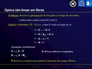
E = - ∂ B/ ∂t ∆ H = Jf + ∂ D/ ∂t ∆ ρf = 0 • ∆ D = B = 0 • ∆ Óptica não-linear em fibras Problema: descreva a propagação de um pulso ao longo de uma fibra conhecendo o pulso inicial E (z=0, t) Solução: determine ∂E / ∂z (i.e., como E varia ao longo de z) Equações constitutivas: D = εoE + P B = µoH + M D, H fluxo elétrico e magnético P descreve a resposta do material à presença do campo elétrico
∆ ∆ ∆ ∆ ∆ Óptica não-linear em fibras Elimina termos magnéticos B e H (εoE + P) H ) = - µo∂2 / ∂t2 ( - ∂ / ∂t ( µo E) = - ∂/∂tB = ∆ ( E) = - 1/c2∂2 E /∂t2 - μo ∂2P/∂t2 ∆ Para resolver para P precisa-se de mecânica quântica. Longe de resonâncias, vale a expansão de Taylor : P = εo [ χ(1)E + χ(2)E•E + χ(3) E•E•E + …] Aproximação de dipolo elétrico (termos do tipo B E, E. E, etc são desprezados) ∆
∆ ∆ Óptica não-linear em fibras ( E) = ( ∆ ∆ •E) - 2 E ∆ Pulse propagation equation ∆ 2 E - 1/c2∂2 E /∂t2 = μo ∂2P/∂t2
P = o (1)E+o(2)E.E+o(3)E.E.E+ ... 2 2 ∂ ∂ 2 E P µo ∆ 1 E ∂ ∂ não-linear linear - t2 t2 = c2 2 2 2 ∂ ∂ ∂ E E E ∂ ∂ ∂ x2 z2 y2 2 ω 2 c Assuma modos transversais: autoestados de propagação Óptica não-linear em fibras Equação de onda para luz em materiais Caso linear: P ~ E Seja Etot = E (z) exp (iωt) + E* (z) exp (-iωt) + + E [1 + χ(1)] = 0 + n2 (depende de ω = dispersão)
n Normal dispersion Anomalous dispersion n decreases with ω ωo ω ωα/c ω Refractive index is well described far from resonances by: Sellmeier equation
∂ E P n2ω2 µo + = ∂ c2 t2 2 ∂ 2 ∆ E ∂ t2 Equação de onda para luz em materiais Solução: Separa variáveis e elimina x e y: E(r,t) = F(x,y) A(z,t) exp [i(βz-ωt)] x Equação transversal: ∂2F/∂x2 + ∂2F/∂y2 + [ε(ω)Ko2 - β2] F = 0 Condições de contorno fazem aparecer modos F(x,y) são funções de Bessel, combinadas em HEmn e EHmn LP01 LP11 LP02
Automodulação de fase Assuma modos transversais: autoestados de propagação P = o (1)E+o(3)E.E.E Seja Etot = E (z) exp (iωt) + E* (z) exp (-iωt) E.E.E= E 3 exp 3(iωt) + 3 E E* E exp (iωt) + 3 E* E E* exp (-iωt) + E *3 exp 3(-iωt) THG I I E.E.E= E 3 exp (i 3ω t) + 3 I E exp (iωt) + cc O termo não-linear pode ser expresso como uma correção de n P = o (1)E+(3 o (3) I.) E (n0 + n2I) Índice de refração depende da intensidade
Consequências da automodulação de fase • o índice de refração é alterado pelo próprio pulse de luz • SPM depende da intensidade do pulso • Na presença de SPM a onda se adianta ou se atrasa • Isto se traduz na mudança da frequência do pulso • O espectro se alarga: as caudas não sofrem SPM • o pico sofre SPM, λ muda No SPM λ t SPM λ
Óptica não-linear em fibras Pulso = cos (ωot-kz) Fase instantânea = (ωot-kz) = (ωot-2πnz/λ) Frequência instantânea ∂Φ/∂z = ωo if n = no ωo-2πn2z/λ dI/dz if n = no + n2I Chirp: varredura de frequências, Desenvolvido durante a 2a guerra para compressão de radar Com SPM o espectro alarga mesmo se a forma do pulso permanecer constante (na ausência de dispersão) Depende de dI/dT, altas intensidades criam um chirp grande
cauda frente Time ω ω+ δω ωo Time ω - δω Automodulação de fase A frente do pulso se torna avermelhada A causa se desloca para o azul Varredura linear onde o pulso é mais intenso Varredura positiva: frequência aumenta Pulsos quadrados só tem SPM durante as rampas Qual é o chirp induzido por um laser CW de 200 W ao longo de uma fibra de 1 km-long devido a SPM?
Automodulação de fase Qualitativamente: porque oscilações? ω Time Mesma frequência, diferentes tempos interferência
Quando um campo intenso é aplicado P =o (1) E+o(2)E.E + o(3)Eappl Eappl E + ... Outros efeitos não-lineares de 3a ordem Em fibras de vidro P = o (1) E+o(2)E.E + o(3)E.E.E + ... Kerr effect Quando um campo DC é gravado (poling) P = o (1) E+ o(2)E.E + o(3) ErecEappl E + ... (2)eff
w w (3) 2 2 w w 2 2 w w c 0 0 w w dc dc w w w w w w w w w w dw dw + + +0 +0 dw dw = = (3) (3) (3) w w w w + + + + dw dw dw dw w w w w w w c c c 0 0 0 0 dc dc dc dc Outros efeitos não-lineares de 3a ordem SHG com campo gravado w w w w w w w w w w w w w w w w w w w w w w w w 2 2 2 2 + + + + + + 0 0 = = = = (3) (3) 2 2 w w 2 2 w w c c 0 0 w w w w dc dc Efeito eletro-óptico com um campo DC gravado
Poling Vidro é um material simétrico P Não exibe não-linearidade de segunda ordem E (2) = 0 in fibras Quebrando a simetria: Grava-se um campo permanente DC! Poling P Apesar de (2) ainda ser zero, E (3) EDC . E . E ~ (2)eff E . E
Gravando o campo elétrico IR, visible (optical poling) Visible + electric field (optical-field assisted poling) UV + electric field (UV poling) Fs + electric field (fs poling) -rays + electric field (gamma-ray poling) Heat + electric field (thermal poling) Ion implantation Heat + electrostatic charging (thermal charging)
Seeded SH Fiber Nd:YAG laser IR. KTP Poling óptico P2ω ~ Eω EωErec SH Fiber Nd:YAG laser IR.
Optical poling Fibra atacada com HF e examinada num microscópio Rede com QPM é gerada pelo campo óptico
w 2 mm 2w Poling térmico + Poling fused silica 280 oC R. Myers, S. Brueck et al, Opt. Lett. 16, 1732 (1991) silica - Strong recorded electric field ~108 - 10 9 V/m ! Top layer < 15 µm Create an effective (2) (3) Edc . E . E ~ (2)eff E . E
High voltage Active arm 280 oC HOT-PLATE ~265 oC 3 dB 3 dB Reference arm Poling sobre um hot-plate
Fibras electroópticas Índice depende fracamente do campo aplicado Antes do poling Só efeito Kerr P = PL + Eω Eappl Eappl Applied field Low amplitude Small phase shift
Erecorded Fibras electroópticas Índice depende do campo aplicado Antes do poling Só efeito Kerr Depois do poling Só efeito Kerr P = PL + EωErec Eappl P = PL + Eω Eappl Eappl Applied field Low amplitude Small phase shift
Erecorded Fibras electroópticas Índice depende do campo aplicado Antes do poling Só efeito Kerr Depois do poling Só efeito Kerr P = PL + EωErec Eappl P = PL + Eω Eappl Eappl Applied field Low amplitude Large phase shift
Caracterização Mach-Zehnder
Componente a fibra polarizada Modulador de fase electroóptico
110 π phase shift Χ(2) = 0.25 pm/V Vπ = 110 V Modulador eletroóptico a fibra Phase modulator Typical values @ 1 µm Vπ ~ 100 V Electrical bandwidth: 20 MHz Loss: 1 dB (fast axis) 10 dB (slow axis) Χ(2) = 0.25 pm/V OE 17, 1553 (2009)
2x2 push-pull fiber switch/modulator 3 dB 3 dB Interferometro Mach-Zehnder a fibra Depois do poling Vπ = 38 V ΔL = L2 – L1 ~ 200 µm
15Vpp Video source 1V Fiber link TV Electrooptical fiber interf. Det. CW laser Transmissão de vídeo Poled fibre modulator for video transmission Acreo – ECOC 2004 exhibition
Coherence length Quasi phase-matching QPM in Xtal SHG Phase matched • Comprimento de coerência: • em cristais ~5 µm • em fibras ~40 µm QPM by Erasure Not phase matched Length
Metal-filled contacted fiber χ Poling creates a uniform (2) in the core Periodic UV erasure Apagamento periódico com UV
Seeded SH Fiber Nd:YAG laser IR. KTP Determinando o período necessário P2ω ~ Eω EωErec SH Fiber Nd:YAG laser IR.
36.1 µm Optical poling Etched fiber under microscope
Fibra poled periodicamente High-average-power second-harmonic generation from periodically poled silica fibers, A. Canagasabey et al, Opt Lett, 15 Aug 2009
Espalhamento Raman Stimulated Raman scattering (Blillouin…) Energy is lost to vibrations (in silica peak ~440 cm-1) Shift from 1.06 µm to 1.12 µm, and then 1.18 µm, 1.24 µm… Shift at 1.48 µm is to 1.58 µm At room temperature, most atoms are in their vibrational ground state Laser excites vibrations (Stokes) Laser de-excites vibrations extremely unlikely (no anti-Stokes peak seen)
Espalhamento Raman Espalhamento Raman estimulado Ganho do espalhamento Raman
∂ E P n2ω2 µo + = ∂ c2 t2 2 ∂ 2 ∆ E ∂ t2 2 Equação de onda para luz em materiais Na aproximação de envelope variando lentamente ∂A/∂z + β1∂A/∂t + i/2 β2∂2A/∂t2 + αA/2 = + i γ|A|2 A Redefine time origin (travel with pulse referential) i∂A/∂z = -iαA/2 + 1/2 β2∂2A/∂T2 -γ|A|2 A γ = n2ωo/cAeff nonlinear coefficient of the fiber (in STF γ ~2/W km) β1 = 1/vG β2 = GVD parameter
i∂A/∂z = -iαA/2 + 1/2 β2∂2A/∂T2 -γ|A|2 A Absorption Dispersion Nonlinearity Como estimar a importância destes efeitos? (Govind rules ok!) LD = To2 /|β2| Comprimento de dispersão LNL = 1/γPo Comprimento de não-linearidade Equação não-linear de Schroedinger (when α~0) i∂A/∂z = 1/2 β2∂2A/∂T2 -γ|A|2 A
i∂A/∂z = 1/2 β2∂2A/∂T2 -γ|A|2 A Normalizing for pulse duration and power t = T/To A(z,t) = √Po exp(-αz/2)U(z,t) i∂U/∂z = ± 1/2LD ∂2U/∂T2 – 1/LNL exp(-αz) |U|2 U (sign of β2) Third order dispersion n(I) leads to ∆β(ω) Self-steepening Delayed material response Raman SFS
Quatro regimes de pulsos Four regimes: 1) L<<LD and L<<LNL no dispersion, no nonlinearity 2) L>LD and L<<LNL dispersion, no nonlinearity 3) L<<LD and L>LNL no dispersion, nonlinearity 4) L>LD and L>LNL dispersion, nonlinearity
LD = To2/β2 large: long pulse (or low dispersion) LNL =1/γPo large: low power (or low nonlinearity) i∂U/∂z = ± 1/2LD ∂2U/∂t2 – 1/LNL exp(-αz) |U|2 U Caso 1 i∂A/∂z = -iαA/2 + 1/2 β2∂2A/∂T2 -γ|A|2 A i∂A/∂z = -iαA/2 time time A = Ao exp(- αz) Pulso apenas se atenua λ λ
Caso 2: dispersão No nonlinearity (intensity or γtoo low) For example, To = 1 ps, Po = 1 mW L>LD and L<<LNL dispersion, no nonlinearity GVD governs propagation: i∂U/∂z = β2/2 ∂2U/∂T2 Solve using Fourier transform The phase depends on the frequency (and propagated distance) Red and blue are phase shifted by different amounts
Caso 2: dispersão red blue time time dispersion λ λ What happens to a chirped pulse when it propagates under a regime dominated by GVD? Predispersed If the pulse is chirped to start with, the pulse duration can narrow due to GVD
Dispersão cromática Chromatic dispersion Broadband optical output Broadband optical input