Download
1 / 19
200 likes | 486 Views
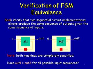
Verification of FSM Equivalence. Goal : Verify that two sequential circuit implementations always produce the same sequence of outputs given the same sequence of inputs. out1. out2. i1. i1. M1. M2. Note: both machines are completely specified.

E N D
Verification of FSM Equivalence Goal: Verify that two sequential circuit implementations always produce the same sequence of outputs given the same sequence of inputs. out1 out2 i1 i1 M1 M2 Note: both machines are completely specified. Does out1 = out2 for all possible input sequences?
M1xM2 M1 i f M2 FSM Equivalence of the Product Machine Form the product machine: M(S,I,T,O,Init) x = (x1,x2) present state y = (y1,y2) next state i = i1 = i2 input Init(x) = (Init1(x1) x Init2(x2)) initial states T(x,i,y) = T1(x1,i,y1) T2(x2,i,y2) transition relation f(x,i) = (f1(x1,i) f2(x2,i)) single outputwhere denotes XNOR operation.
Implicit State Enumeration The FSM’s are equivalent iff for all inputs, their outputs are identical on all reachable state pairs. Let R be the set of all reachable state pairs. Equivalence is verified by the following predicate:(x,i) [(x R) f(x,i)] Easy computation with BDDs. Simply compute+ f(x,i)and check if this is identically 1.
Implicit State Enumeration The followingfixed point algorithm computes the set of reachable state pairs R(x) of an FSM.R0(x) = Init(x)Rk+1(x) = Rk(x) + [y x] x, i (Rk(x) T(x,i,y))where [y x] represents substitution of x for y. The iteration terminates when Rk+1(x) = Rk(x) and the least fixed point is reached.
Implicit FSM Traversal Implicit enumeration of reached state set • manipulates set of states directly in a BFS manner • exponential speed-up over explicit enumeration methods (sometimes) • exploits the fact that the number of states does not usually reflect system complexity • implicit state enumeration may take a long time for sequentially deep circuits e.g. those with counters one set of states at a time: one step
Finding Reachable States in an FSM R0 is the set of intial states R0
R0 Finding Reachable States in an FSM R1 is the set of states reachable from the initial states in less than or equal to one steps. R1
R1 R0 Finding Reachable States in an FSM R2 is the set of states reachable from the initial states in less than or equal to two steps. R2
R1 R0 Finding Reachable States in an FSM The fixed-point iteration terminates after finding R4 = R5. The resultant set is the set of reachable states. R2 R4=R5
Partial Product Method Do not need to compute the transition relation T(x,i,y) explicitly as a single monolithic BDD. Can keep T(x,i,y) in product form(called “partitioned translation relation”):
Partial Product Method Using Constrain Can form the constrain with respect to Rk(x) of each (yj fj) before forming the final AND. This usually reduces the size of the final AND. The final AND operation can be decomposed into a balanced binary tree of Boolean ANDs. • intermediate variables can be quantified out as soon as no other product depends on those variables.
Using Constrain Can pre-cluster groups of Tj(xj,ij,yj) (defined as (yj fj(xj,ij))) together:Cj = ikj(Tj1,...,Tjk)where the ikj that we can quantify out here are the ones that do not appear in any other Ti. Thus Using constrain is a bad idea since (Cj(xj,ij,yj))Rk(x) may result in a BDD with more variables. (It is better to use RESTRICT).
Better Idea: Use Restrict Linearly order (heuristically) the Cj and multiply from the right by Rk(x) one at a time, quantifying variables xq, iq as soon as possible (when they appear in no other terms). Ri+1 = Ri(x) + [y x] (xp,ip)Cl1(...((xq,iq )ClqPi(x))...) where Pi(x) = RESTRICT(Ri, ). Note: here we do not care about any state in Ri-1 since we have already found all successor states of these. Computation done as a binary tree where quantification of x and i is done as soon as possible: Quantify all remaining variables that appear in no other remaining node. ClqPi(x)
Restrict Operator Restrict: • if f is independent of xi then RESTRICT(f,c) is also. • it does not have the other nice properties of constrain. • Experiments show that restrict produces smaller BDDs. function RESTRICT(f,c) assert(c 0) if (c = 1 or is_constant(f)) returnf else if (cx’i = 0), returnRESTRICT(fxi,cxi) else if (cxi = 0), returnRESTRICT(fx’i,cx’i) else if (fxi = fx’i), returnRESTRICT(fxi, cxi + cx’i) else returnxiRESTRICT(fxi,cxi) +x’i RESTRICT(fx’i,cx’i)
Recursive Image Method (Ri-1 is the set of currently reached states and g is the vector of next state functions) The method uses CONSTRAIN: Let g : Bn Bm, g = [g1, g2, ..., gm], and c = characteristic function of Ri-1 . First step: use the CONSTRAIN operator to form f = gc = [(g1)c, (g2)c, ..., (gm)c]. Second step: the range of f is determined. Let R(f) denote the range of the function f. Ri = R(f)(y) = y1R([f2,...,fm]f1) + y’1R([f2,...,fm]f’1)
Explicit FSM Traversal Explicit enumeration: • process one state at a time • for each state, next states are enumerated one by one • complexity depends on the number of states and the number of input values. • methods that enumerate the state space explicitly cannot handle FSM’s with a large number of states first one state at a time 1 second 2 third 3 fourth 4
State enumeration State traversal techniques are essential to: • synthesis of sequential circuits • verification of sequential circuits Applications: • sequential testing [Cho, Hachtel and Somenzi ITC ‘91] • extraction of sequential don’t cares • implementation verification: • checking sequential equivalence [Coudert and Madre ICCAD ‘90][Touati, Lin, Brayton and Sangiovanni ICCAD ‘90] • design verification: • checking language containment of -regular languages [Touati, Kurshan and Brayton 1991] [HSIS system ‘94] • CTL model checking [Burch, Clarke, McMillan and Dill DAC ‘90] [SMV (CMU ‘91), VIS (Berkeley ‘96), MOCHA (Berkeley ‘98) systems]