Download
1 / 34
340 likes | 366 Views
Explore the innovative computational physics curriculum at Illinois State University, integrating theoretical framework with cutting-edge computational techniques. From computer coding to advanced skills, experience a comprehensive physics education.

E N D
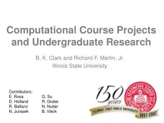
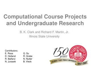
B. K. Clark and Richard F. Martin, Jr. Illinois State University Computational Course Projects and Undergraduate Research Contributors: E. Rosa Q. Su D. Holland R. Grobe R. Balfanz N. Nutter N. Jurasek B. Vleck
Resources: ISU Physics and its Peers 2004 - 2006 Institution # of faculty publications % of faculty average grant % of faculty per faculty with publication amount with grant Top 10 68 6.62 64 % $ 569 K 11 % ISU Physics 12 4.83 83 % $ 92 K 17 % Top 10 Physics departments Cal Tech, Harvard, Cornell, JHU, UC Berkeley, NYU, Michigan, Duke, Stanford, UIUC From: “Chronicle of Higher Education” 1/12/2007 www.chronicle.com/stats/productivity
Undergraduate physics research at ISU Nonlinear Dynamics Nanoscience Space Physics Atomic, Molecular, and Optical Physics Biophysics
Annual Average Number of Graduates 2002-2004 United States Air Force Academy 24 Harvey Mudd College 22 U. of Wisconsin – La Crosse 22 Illinois State University 20 Source: American Institute of Physics ISU Computer Physics Sequence 1998-2007 Total graduates 35 Graduates per year 4 Computation Research Mentors 9 Advanced Computational Physics Modules 7 (3 per year) Number of physics graduates from 1980 to present CPY: Computer physics PTE: Physics Teaching PHY: Physics ENG: 3/2 program
Computer Physics Curriculum Frontiers in Physics Physics for Scientists and Engineers I Physics for Scientists and Engineers II Physics for Scientists and Engineers III Methods of Theoretical Physics Mechanics I Electricity and Magnetism I Experimental Physics Quantum Mechanics I Thermal Physics Elective Courses One additional 300-level Physics course. Recommended Electives Nonlinear Science Molecular Dynamics Simulations Methods of Computational Science Advanced Computational Physics Computational Research in Physics At least one from: PHY 320 Mechanics II PHY 340 Electricity and Magnetism II PHY 384 Quantum Mechanics II Computer Science Courses Programming for Scientists Hardware and Software Concepts
Computer skills and techniques Techniques introduced in the core for both computer physics and physics majors 2D graphics: 6-8 Mathematica: 2-3 Function Evaluation: 2+ Data analysis/curve fitting: 3 ODE – Euler, 2 ODE – 2nd Order Methods: 3 Monte Carlo (simple): 4 ODE – 4th order Runge-Kutta: 3 Fourier: 4-5 Integration: 1+ Over relaxation: 1-2 Graphical analysis of transcendental equations: 1-2 Molecular Dynamics: 1-3 Phy 320, 340, 384 Complex Analysis: 1 Monte Carlo (variational): 1 Eigenvalues: 2 Molecular Dynamics:1-3 Other elective courses Surface-of-section: 1 Ray Tracing: 1 Matrix methods: 1 Fractal Dimension: 1
Computer skills and techniques Methods of Computational Science ODE – Adaptive/High Order: 1-3 Computational efficiency: 1 Integral equations by matrix inversion: 1 Theory of ODE techniques:1 Computational Research in Physics Mesh Method for Liouville eqn Quadratic Programming and optimization Matrix methods Cellular Automata Integral equations by matrix inversion Neural network Eigen analysis Each student has seen one of these in the recent past Advanced Computational Physics Split operator: 1 Finite element: 1 Neural network: 1 Molecular Dynamics: 1-3 Monte Carlo: 1-4 Students see at least three of these Number indicates the number of times a student is likely to encounter a skill or technique. Listings for advanced courses do not include all of the techniques a student has previously encountered.
Observations on computer physics at ISU Computational physics is on an equal footing with experimental and theoretical physics at ISU. This will probably be the norm in another generation. When computational techniques were introduced across the program in the late 80’s and early 90’s, faculty teaching each course chose which techniques to include in their respective courses. Some general discussion occurred in an attempt to make sure that students encountered a broad range of techniques and techniques deemed critical, in particular. The computer physics sequence started in 1998. Methods of Computational Science is designed to provide a theoretical framework for computational techniques. Computational Research in Physics evolved from an earlier course and provides students with a mixture of theoretical physics and related cutting edge computational techniques. The program at ISU focuses on students writing their own computer code. There are some exceptions. In a few instances a faculty member provides a working code and students must make some changes. The department also uses Mathematica.
Most faculty actively contribute to the integration of computer physics into the curriculum. Some have been encouraged to boost the level of computer physics in core courses. In informal discussion with 3rd semester physics students, teacher education students generally prefer less computer physics integration, computer physics students really like it, and traditional physics students fall somewhere in between. By graduation, each student has selected the course of study most appealing to him or her, and each program is responsible for about a quarter of our graduates. Computer physics and traditional physics students generally agree that computational physics has helped them to more clearly understand equations and systems. The Computer physics sequence at ISU thrives in part because 75% of faculty classify themselves as computational (at least in part), providing a strong base. All faculty support the program. Computational physics is more financially accessible to under-funded state schools than experimental physics.
Physics 388 Advanced computational physics Neural networks Comparison of classical and quantum physics Bio-optical physics Finite element analysis Physics 390 Computational research in physics Computational study of synchronization of coupled non-linear oscillator systems Gerrymandering and fractal dimensions of congressional districts Cellular automaton investigation of the transition from non-flocking to flocking behavior Central current sheet ion distribution functions
Neural Networks • Interdisciplinary field active since 1940’s • Used regularly in science and engineering for prediction, optimization, data mining, etc. • Pedagogical goals: students will • Understand neural models • Build intuition for selecting net parameters • Reinforce basic timeseries analysis (e.g. power spectrum & autocorrelation function) • Understand when to train with causal inputs (physics example) vs. self-prediction (financial example) • Write ANN code to do self-prediction with Dow Jones index • See at least one associative or self-organizing network model
Neural Networks • Scientific ANN example: the Auroral Electrojet (AE) Index • Fast decorrelation time so use causal inputs • Train with several different sets of input data to determine which sets • allow best prediction • Example: Single hidden layer net, using backpropagation • [Gleisner & Lundstedt. 1997] Results consistent with years of data analysis Go over network design choices
Neural Networks • ANN Topics • Biological NNs, learning theory • Neuron models, training, limitations • Learning rules: Hebb, Delta, Backpropagation • Net design: theorems, rules of thumb, testing • Predictability of timeseries • Backpropagation for timeseries (AE and financial) • Hopfield nets: character recognition Predict Dow Jones Train with 200 months Predict for 300 months • Written Assignments • Basic neuron models • Linear separability • Programs • Single neuron for NOR • Delta rule for XOR • Backpropagation for time series, DJIA
Comparison of Classical and Quantum Physics(based on research program of R. Grobe and Q. Su) • Classical and quantum physics are employed to describe many phenomena. Understanding their range of applicability is important in developing students physics intuition • Pedagogical goals: students will • Simulate non-interacting classical ensembles with a Monte Carlo technique • Use non-uniformly distributed random numbers, Box-Muller algorithm, rejection method, and Fast Fourier transformation • Use Split-operator techniques • Create an NCAR graphics animation • inputs (physics example) vs. self-prediction (financial example)
Comparison of Classical and Quantum Physics Students calculate spreading of a classical ensemble of particles and wave function that describes the equivalent quantum mechanical picture. The particles experience a constant (linear) force. Classical results: particle distribution in phase space at three times Quantum results: wave function at three times
Comparison of Classical and Quantum Physics • Topics in Classical and Quantum Topics • Distribution functions, average values, higher moments • The Liouville equation, multi-particle simulations • The Schrödinger equation, exploiting linearity, decomposition into advantageous states • Free-time evolution using FFT • Second and Third order split-operator scheme with error estimates • Written Assignments • Calculate moments of a swarm of bees • Liouville equation and the conservation of the norm of r • Programs • Evolution of a classical distribution of particles • Evolution of a quantum mechanical wave packet
Bio-Optical Physics(based on research program of Q. Su and R. Grobe) • One of the youngest fields and expected to play a significant role in the “century of life sciences” • Non-invasive optical diagnostic techniques are expected to have great impact on the economics of medicine and help provide early detection of cancers • Pedagogical goals: students will • Understand the physics of x-ray and IR imaging • Understand the micro- and macroscopic pictures of light/matter interactions • Apply the Boltzmann equation to light scattering using Monte Carlo techniques • Model the propagation of light through a turbid medium
Bio-Optical Physics Transmission and reflection of modulated beam Beam spread for constant intensity Beam spread for modulated intensity
Bio-Optical Physics Topics in bio-optical physics Introduction to bio-optical physics A matrix model of X-ray image reconstruction Micro- and macro-scopic views of light-tissue interactions The Boltzmann equation (BE) for light The scattering phase functions A bi-directional model of light scattering A Monte-Carlo algorithm to solve the BE The photon density waves The diffusion approximation Imaging with mirrors Written Assignments X-ray shadow gram absorption coefficients 1-D diffusion equation Programs 1-D Boltzmann equation via a Monte-Carlo algorithm Photon density waves with constant and periodic time dependence
Finite Element Analysis Powerful numerical method for solving problems in physics and engineering such as: fluid flow, heat transport, structural mechanics (torsion, elasticity, etc.) Frequently used in engineering for modeling problems such as the structural framework of automobiles and aircraft, groundwater flow, and heat flow. Easily generalized to handle 1D, 2D and 3D problems with complicated boundaries, sources, sinks, and multiple materials.
Finite Element Analysis • Pedagogical goals: students will • Understand the theoretical basis for the finite element method, i.e. minimization of a functional on a grid. (Calculus of Variations.) • Understand how to set up the element grid in 1 and 2 dimensions. • Write a 1-D finite element code for calculating the temperature in a fin with various boundary conditions (e.g. insulated/non insulated) and with varying materials. • Topics in Finite Element Analysis • Fundamental concepts • Nodes, elements, shape functions • Calculus of variations • Functionals • Heat transfer • Embedding equations
Finite Element Analysis • Written Assignments • Calculate various shape functions • Determine single element equation matrices • Determine embedding equations • Programs • Solve 1-D heat transfer along a fin (circular rod) Example results for a 1-D uninsulated rod of radius 1cm and length 10 cm. The ambient air temperature is 30 C and the thermal conductivity of the material is 75 W/cm-C. There is a continuous heat input of 450 W/cm2 on the left end of the rod. Calculation in done using 10 elements.
Chua Circuit and Chaotic Attractors Computational Study of Synchronization ofCoupled Non-Linear Oscillator Systems (a component of E. Rosa research program) Student: Brian Vlcek Advisor: E. Rosa dx/dt = (G(x2-x1)-y(x1))/C1 dy/dt = (G(x1-x2)-x3)/C2 dz/dt = -x2/L G = 1/R Phase difference: Δj12 = j1 - j2
fast medium slow Computational Simulation: Chua Circuit Power Spectra ε12 = ε13 = 0.0 ε12 = 0.055 ε13 = 0.010
Neural Action Potential Simulation Hodgkin-Huxley Neural Spiking Model ε12 = ε13 = 0.0 ε12 = ε13 = 0.01
Chicago Congressional Districts Gerrymandering and Fractal Dimensions of Congressional Districts Student: Nicholas Jurasek Advisors: B. Clark, D. Holland Written in C++ Uses SDL image library for image manipulations It has a very easy to use point and click interface. Very fast, can calculate the fractal dimension in seconds.
Box Counting Algorithm The program loads in a BMP image, then displays it on the screen. The user then clicks on the boarder Color. A district color is then selected. The program then breaks the image into boxes and looks in each box to see if it contains both the border color and the district color. If a box meets both conditions it is on the perimeter of the district, and it is counted. The number of boxes is then plotted against the box dimension. The boxes are then decreased in size by a factor of 2 and the process is repeated. After several iterations the slope of the emerging line is calculated and this becomes the fractal dimension.
Cellular automaton based investigation of the transition from non-flocking to flocking behavior Student: Ryan Balfanz Advisors: D. Holland, B. Clark • Flocking can be simulated from a few simple “microscopic” rules (Reynolds) • W1, Flock Centering: head to the center of the other boids • W2, Collision Avoidance: don’t fly into other boids • W3, Velocity Matching: approach the average velocity of the other boids • By applying the rules to each boid, a macroscopic behavior emerges • What causes the transition between non-flocking and flocking motion?
vinitial v1* w1 vfinal v2* w2 v3* w3 Typical behavior encountered for 16 boids No Organization Bird Flocking
Typical behavior encountered for 16 boids vinitial v1* w1 vfinal v2* w2 v3* w3 Vortex Fish Swarm
Central current sheet ion distribution functions (a component of D. Holland research program) Student: Nathan Nutter Advisor: D. Holland Ions interacting with the magnetotail have complicated trajectories resulting in a relative redistribution of particles as compared to their incident distribution.
Current sheet algorithm Use a test particle code to push a distribution of particles through a model magnetic field. Each particle should contribute equal phase space “weight” in the uniform magnetic field region. Create single particle distribution by putting the particle in its proper energy/pitch angle/z-position bin at each time step. fi (H,,z) Divide the single particle distribution by the total number of “counts” in the top grid cell so that each particle contributes unit density to the total distribution. Sum the single particle distributions to get an overall distribution.
Typical results for current sheet Since individual particles are non-interacting, this is an ideal problem for parallel processing. (xgrid)