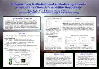
Latitudinal gradients
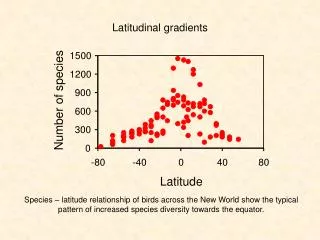
1500. 1200. 900. Number of species. 600. 300. 0. -80. -40. 0. 40. 80. Latitude. Latitudinal gradients. Species – latitude relationship of birds across the New World show the typical pattern of increased species diversity towards the equator. Coral reef fish. Labridae.

Latitudinal gradients
E N D
Presentation Transcript
1500 1200 900 Number of species 600 300 0 -80 -40 0 40 80 Latitude Latitudinal gradients Species – latitude relationship of birds across the New World show the typical pattern of increased species diversity towards the equator.
Coral reef fish Labridae Pomacentridae Mora et al. 2003 Diversity of coral reef fish declines from their centres of diversity. There is also a strong correlation between distance and duration of the pelagic phase, which is a proxi of dispersal ability.
Latitudinal gradient in species diversity of mollusks on North and South American Pacific shelves (Valdovino et al. 2003) • Centers of diversity are often shifted north or south • Species richness sharply declines towards temperate regions • Tropics contain a very large proportion of total species richness • Species near the center of species richness are often less dispersive
The general patterns Hillebrand (2004) conducted a meta-analysis about 581 published latitudinal gradients • Basic conclusions • Nearly all taxa show a latitudinal gradient • Body size and realm are major predictors of the strange of the latitudinal gradient • The ubiquity of the pattern makes a simple mechanistic explanation more probable than taxon or life history type specific
Counterexamples The sawfly Arge coccinea, Photo by Tom Murray Soybean aphid, Photo by David Voegtlin The ichneumonid Arotes sp., Photo by Tom Murray The aquatic macrophyte Hydrilla verticilliata, Photo by FAO These taxa are most species rich in the northern Hemisphere
Some theories that try to explain observed latitudinal gradients in species diversity. Older theories: Circular explanations: Environmental stability Competition ( Dobshansky 1950) or predictability Predation ( Klopfer 1959) Paine 1966) Productivity Niche width ( Slobodkin and Sanders 1969) (Ben Eliharu and Safriel 1982) Heterogeneity Host diversity ( Pianka 1966) Latitudinal decrease in (Rhode 1989) angle of sun Epiphyte load ( Terborgh 1985) (Strong 1977) Aridity Population size ( Begon et al.. 1986) ( Boucot 1975) Seasonality ( Begon et al.. 1986) Number of habitats ( Pianka 1966) Latitudinal ranges ( Rapoport 1982) Time related explanations: Area (Connor and McCoy 1979) Temperature dependence of Range size related explanation: (Alekseev 1982) chemical reactions Random range sizes Temperaturedependent mutationrates (Colwell and Hurtt 1994) (Gillooly et al. 2005) Evolutionary time Energy related explanations: ( Pianka 1966) Energy supply Ice age refuges (Rhode 1992) ( Pianka 1988)
Habitat heterogeneity North American grasshoppers Red data points: Multihabitat gradient in ant species diversity Blue data points: Gradient for one habitat type Latitudinal gradients can also be found within single habitat types Energy or area per se Ant species richness is significantly correlated to mean annual temperature and mean primary production, but not to area
Refuge theory The refuge theory of Pianka tries to explain the gradient in species diversity from ice age refuges in which speciation rates were fast. This process is thought to result in a multiplication of species numbers in the tropics. In the temperate regions without refuges species number remained more or less constant.
Biodiversity and temperature Western Atlantic gastropods Eastern Pacific gastropods Species diversity of marine gastropods is significantly correlated with mean surface water temperature
Metabolic theory and species latitudinal gradients in species richness The inverse of time are rates. Examples: Growth rates, mutation rates, species turnover rates, migration rates Hence biological rates should scale to body weight and temperature by Biological times should scale to body weight to the quarter power Examples: Generation time, lifespan, age of maturation, average lifetime of a species Body weight corrected energy use should exponentially scale to the inverse of temperature. The slope –E/k should be a universal constant for all species independent of body size.
The rate of DNA evolution predicted from metabolic theory Body size specific metabolic rate M/W should scale to the quarter power to body weight and exponentially to temperature Now assume that most mutations are neutral and occur randomly. That is we assume that the neutral theory of population genetics (Kimura 1983) DNA substitution rate a should be proportional to M/W • Body weight corrected DNA substitution rates (evolution rates) should be a linear function of 1/T with slope –E/k = -7541 • Higher environmental temperatures should lead to higher substitution rates (faster evolution) • Body weight corrected DNA substitution rates (evolution rates) should decrease with body weight • Large bodied species should have lower substitution rates (slower evolution)
Diversity and temperature The energy equivalence rule The average abundance N of an assemblage of S species and J individuyals in areal A is N=J/SA • Species richness should increase with environmental temperature • Species richness should increase with energy • The slope of this relationship should be -E/k = -7541K • Caveats: • Mean abundance per unit area is independent of temperature. • The energy equivalence rule holds at least approximately and its slope is independent of temperature. For standard areals and species of similar body size holds therefore
Costa Rican trees along an elevational gradient North American trees North American amphibians Ecuadorian amphibians Prosobranchia species richness Ectoparasites of marine teleosts Fish species richness
Today’s reading Latitudinal gradients: http://en.wikipedia.org/wiki/Latitudinal_gradients_in_species_diversity Gaston K. 2000 - Global patterns in biodiversity - Nature 405: 220-227 Allen A. P., Brown J. H., Gillooly J. F. 2002. Global biodiversity, biochemical kinetics, and the energy equivalence rule. Science 297: 1545-1548.