Download
1 / 36
360 likes | 567 Views
Motion Computing in Image Analysis. - Mani V Thomas CISC 489/689. Roadmap. Optic Flow Constraint Optic Flow Computation Gradient Based Approach Feature Based Approach Estimation Criterion Block Matching algorithms Conclusion.

E N D
Motion Computing in Image Analysis - Mani V Thomas CISC 489/689
Roadmap • Optic Flow Constraint • Optic Flow Computation • Gradient Based Approach • Feature Based Approach • Estimation Criterion • Block Matching algorithms • Conclusion Some slides and illustrations are from M. Pollefeys and M. Shah
Importance of Visual Motion • Apparent motion of objects on the image plane is a strong cue to understand structure and 3D motion • Biological visual systems infer properties of the 3D world via motion • Two sub-problems of motion • Problem of correspondence estimation • Which elements of a frame correspond to which elements of the next frame • Problem of reconstruction • Given the correspondence and the camera’s intrinsic parameters can we infer 3D motion and/or structure Courtesy: E. Trucco and A. Verri, “Introductory techniques for 3D Computer Vision”
Apparent Motion • Apparent motionof objects on the image plane • Caution required!! • Consider a perfectly uniform sphere that is rotating but no change in the light direction • Optic flow is zero • Perfectly uniform sphere that is stationary but the light is changing • Optic flow exists • Hope – apparent motion is very close to the actual motion Courtesy: E. Trucco and A. Verri, “Introductory techniques for 3D Computer Vision”
Optic Flow Computation • Two strategies for computing motion • Differential Methods • Spatio temporal derivatives for estimation of flow at every position • Multi-scale analysis required if motion not constrained within a small range • Dense flow measurements • Matching Methods • Feature extraction(Image edges, corners) • Feature/Block Matching and error minimization • Sparse flow measurements Courtesy: E. Trucco and A. Verri, “Introductory techniques for 3D Computer Vision”
Optic Flow Computation • Image Brightness Constancy assumption • Let E be the image intensity as captured by the camera • Using Taylor series to expand E • Apparent brightness of moving objects remains constant
Optic Flow Computation • Image Brightness Constancy assumption • Apparent brightness of moving objects remains constant • The are the image gradient while the are the components of the motion field Courtesy: E. Trucco and A. Verri, “Introductory techniques for 3D Computer Vision”
Aperture Problem • We can measure • Terms that can be measured • Terms to be computed • Number of equations - 1 • The component of the motion field that is orthogonal to the spatial image gradient is not constrained by the image brightness constancy assumption • Intuitively • The component of the flow in the gradient direction is determined • The component of the flow parallel to an edge is unknown Courtesy: E. Trucco and A. Verri, “Introductory techniques for 3D Computer Vision”
Different physical motion but same measurable motion within a fixed window
Roadmap • Optic Flow Constraint • Optic Flow Computation • Gradient Based Approach • Feature Based Approach • Estimation Criterion • Block Matching algorithms • Conclusion Some slides and illustrations are from M. Pollefeys and M. Shah
Optic Flow Constraint • How to get more equations for a pixel? • Basic idea: impose additional constraints • Most common is to assume that the flow field is smooth locally • One method: pretend the pixel’s neighbors have the same (u,v) • If we use a 5x5 window, that gives us 25 equations per pixel!
Lucas-Kanade Optic Flow • We now have more equations than unknowns • Solve the least squares problem • Minimum least squares solution (in d) is given by • First proposed by Lucas-Kanade in 1981 • Summation performed over all the pixels in the window
Lucas-Kanade Optic Flow • Lucas-Kanade Optic flow • When is the Lucas-Kanade equations solvable • ATA should be invertible • ATA should not be too small (effects of noise) • Eigenvalues of ATA, 1 and 2 should not be small • ATA should be well conditioned • 1/2 should not be large (1 = larger eigenvalue)
Edge • Gradient is large in magnitude • Large 1 but small 2
Low texture region • Gradients has small magnitude • Small 1 and small 2
High texture region • Gradients are different with large magnitudes • Large 1 and large 2
Improving the Lucas-Kanade method • When our assumptions are violated • Brightness constancy is not satisfied • The motion is not small • A point does not move like its neighbors • Iterative Lucas-Kanade Algorithm • Estimate velocity at each pixel by solving Lucas-Kanade equations • Warp H towards I using the estimated flow field • use image warping techniques • Repeat until convergence
u=1.25 pixels u=2.5 pixels u=5 pixels u=10 pixels image H image H image I image I Gaussian pyramid of image H Gaussian pyramid of image I Iterative Lucas-Kanade method
warp & upsample run iterative L-K . . . image J image H image I image I Gaussian pyramid of image H Gaussian pyramid of image I Iterative Lucas-Kanade method run iterative L-K
Roadmap • Optic Flow Constraint • Optic Flow Computation • Gradient Based Approach • Feature Based Approach • Estimation Criterion • Block Matching algorithms • Conclusion Some slides and illustrations are from M. Pollefeys and M. Shah
Feature Based Method • Feature Extraction • Maxima in first derivative of the Image • Local peak in the first derivative • Numerical Approximation • Compute the motion parameters from the best bipartite graph • Correspondence between the feature points in one image with those in the other For more information: Ramesh Jain, Rangachar Kasturi, Brian Schunck: Machine Vision 1995 (140 - 159)
Roadmap • Optic Flow Constraint • Optic Flow Computation • Gradient Based Approach • Feature Based Approach • Estimation Criterion • Block Matching algorithms • Conclusion Some slides and illustrations are from M. Pollefeys and M. Shah
Estimation Criterion • Pixel domain Criterion • MAE/MSE • Lorentzian • Correlation • Frequency Domain Criterion • Cross Correlation • Phase Correlation
Estimation Criterion(contd.) • Pixel Domain Criterion • Estimation criterion aim at minimizing • prediction error is sensitive to noise if number of pixels is not large or if region is poorly textured • Common choice of estimation criterion • Quadratic function is not good since a single large error can bias the estimate of the field • Absolute value function is better than the quadratic since cost grows linearly with error • Does not require multiplications and is better suited for real-time video encoders
Estimation Criterion(contd.) • A more robust criterion is based on the Lorentzian function • Grows slower than |x| for larger errors • Similarity measure using Correlation • Computationally complex because of the multiplications • This criterion requires maximization • Usually the normalized Cross correlation is computed For more details: M. Black, “Robust Incremental Optical Flow”
Estimation Criterion(contd.) • Frequency Domain Criterion • Amplitudes of both the FT are independent of z • Argument difference depends linearly on translation • Global motion is recovered by evaluating the phase difference over a number of frequencies and solving the resulting system of equations • In practice, this method will work only for a single object moving across a uniform background
Estimation Criterion(contd.) • Phase Correlation • In the case of a single global translation, the correlation surface becomes a Kronecker delta function • In practice, there are numerous peaks which correspond to the dominant displacements between the two images • The locations are relatively independent to illumination changes
Roadmap • Optic Flow Constraint • Optic Flow Computation • Gradient Based Approach • Feature Based Approach • Estimation Criterion • Block Matching algorithms • Conclusion Some slides and illustrations are from M. Pollefeys and M. Shah
Block Matching Algorithms • Sparse motion measurements • Motion is spatially constant and temporally linear over a rectangular region of support • The minimization problem is • is an M x N block of pixels with the top-left corner co-ordinate at
-p N -p N M M p p Current Picture Reference Frame v -p N (x,y) (x+u,y+v) M -p p u p Block Matching Algorithms(contd.)
Block Matching Algorithms(contd.) • Principle of Locality of Reference • Block Matching algorithms • Exhaustive Search • Always finds the “deepest” minimum • Computationally very expensive • If I x J is the picture resolution and rate is F fps the overall operations in comparing MxN blocks would be • This corresponds to 29.89 GOPS for p=15 at 30fps for a 720x480 image (3 operations per pixel of one subtraction, one absolute value and one addition)
Block Matching Algorithms(contd.) • Logarithmic Search • Sub-optimal and may get trapped in a local minima • Computationally feasible for real-time video encoders • Search Method • Divide the search space at [-p/2, -p/2] • Search at (0,0) and at 8 major points at the perimeter of the rectangle at [-p/2, -p/2] • Using best match position as starting point, search in the eight perimeter points at the half distance window • If I x J is the picture resolution and rate is F fps the overall operations in comparing MxN blocks would be • This corresponds to 1.03 GOPS for p=15 at 30fps for a 720x480 image For more information refer the work by Dr. Lai-Man Po and C. K. Cheung (http://www.ee.cityu.edu.hk/~lmpo/publications/index.html)
Block Matching Algorithms(contd.) • Hierarchical Search • Sub-optimal for regions containing detail and increased storage requirements • Computationally feasible for real-time video encoders • Search method • Form several low resolution images by low pass filtering • At the lowest resolution perform a sub-optimal search like log search • Propagate search vectors to higher resolution images and perform search • If I x J is the picture resolution and rate is F fps the overall operations in comparing MxN blocks would be • This corresponds to 507.38 MOPS for p=15 at 30fps for a 720x480 image
Conclusion • Motion estimation • Aperture problem • Different algorithms to perform motion analysis • Lucas-Kanade algorithm • Estimation criterion for motion field computation • Block Matching Algorithms • Computational complexity of motion analysis