Download
1 / 44
450 likes | 662 Views
Examining the balance between optimising an analysis for best limit setting and best discovery potential. Gary C. Hill, Jessica Hodges, Brennan Hughey, Mike Stamatikos. University of Wisconsin, Madison. PHYSTAT 2005, Oxford. The problem?. What is an optimal analysis?

E N D
Examining the balance between optimising an analysis for best limit setting and best discovery potential Gary C. Hill, Jessica Hodges, Brennan Hughey, Mike Stamatikos University of Wisconsin, Madison PHYSTAT 2005, Oxford
The problem? • What is an optimal analysis? • Do we go for best sensitivity (lowest upper limit) or for best discovery potential (high deviation away from background expectation)? • How do we optimise for each? • How does choosing one optimisation affect the potential of the other?
Sensitivity • Sensitivity – choose cuts so that the average limit on the physics quantity is minimised • “Model Rejection Potential” • Gary C. Hill and Katherine Rawlins, Astroparticle Physics 19 393 (2003) • Standard optimisation for AMANDA and IceCube
Assessing sensitivity Choose cuts – leaves the signal region, where we will look for an effect above background
OPTIMISATION INDEPENDENT OF ASSUMED SOURCE STRENGTH!
Example : sensitivity of IceCube to diffuse extraterrestrial neutrinos
What about discovery potential? • Suppose one was interested in discovering something and not just setting best limits? • Would the optimisation be different? • What would one optimise?
Characterising discovery* A “discovery” is a rejection of the background only hypothesis at a very high confidence level Of course, a small chance probability does not prove the truth of some alternative hypothesis - unlikely data under a background hypothesis doesn’t mean that some alternative hypothesis is true… P(n|H0) small doesn’t mean P(H1|n) is non-zero!
* To give credit where it is due! • When I submitted this abstract, Louis Lyons mentioned that there was a paper from Giovanni Punzi, PHYSTAT2003, on this question • I had been at that talk and glanced at the paper a long time ago… but obviously things didn’t sink in totally… • Upon reading again, I realised that G.P. had come up with the same basic concept of a “least detectable flux” that one chooses cuts to minimise, that I will talk about and use here
Characterising discovery* A “discovery” is a rejection of the background only hypothesis at a very high confidence level Of course, a small chance probability does not prove the truth of some alternative hypothesis - unlikely data under a background hypothesis doesn’t mean that some alternative hypothesis is true… P(n|H0) small doesn’t mean P(H1|n) is non-zero!
Chance probabilities fordifferent sigmas John Kelley, UW Madison, with Mathematica
How likely are we to see such low chance probabilities if there really is a signal?
Least detectable signal vs background Solid lines: average upper limit curves, 68, 90, 95, 99%
MRF → MDF • Least detectable signal curves replace average upper limit curves • Compare minima for limits and discovery
Neutrino Beams: Heaven & Earth NEUTRINO BEAMS: HEAVEN & EARTH Black Hole Radiation Enveloping Black Hole p + g -> n + p+ ~ cosmic ray + neutrino -> p + p0 ~ cosmic ray + gamma
Atmospheric Muons & Neutrinos astrophysicaln • “Atmospheric muons” from cosmic ray showers, penetrating to the detector from above • “Atmospheric neutrinos” from the same air showers, forming a diffuse background and calibration beam • Astrophysical neutrinos: interesting signal cosmic ray atm. n 10-4 Hz cosmic ray 102 Hz atm.m
South Pole Dome road to work AMANDA Summer camp 1500 m Amundsen-Scott South Pole station 2000 m [not to scale]
Astrophysical point source search • Know sky position of the source from other wavelength observations. • e.g. VHE gamma-ray people look where the x-ray people saw something, neutrino people look where the gamma-ray and/or x-ray people were successful
Reconstruction angular resolution:point spread function differential, weighted with solid angle differential Gaussian signal uniform background Reconstruction response: Gaussian in angle away from true arrival direction
integrated signal and background LDS, 5-σ signal aul 90% background
Solid : best dashed : best MRF dotted : best MDF Curves of MRF, MDF MDF MRF
bg = 10-4 inside 1 degree
bg = 0.1 inside 1 degree
bg = 1 inside 1 degree
bg = 10 inside 1 degree
bg = 30 inside 1 degree
best MDF/MRF angular cut vs log10 background both MRF and MDF cut converge toward best b/s cut – 1.58 times resolution – historical “standard” choice of astrophysics community
Comparison of the MDF/MRF performance Difference between best MRF cut and best MDF cut For larger backgrounds, don’t lose much on MRF by choosing to optimise for MDF and vice versa. At very low backgrounds, choose more carefully (discrete Poisson strikes again!)
More to check? • Different confidence levels • how do optimisations vary with confidence levels? • should we use consistent levels in limit and discovery optimisation? • Different power settings • independent of power in some cases • not true generally • is there a general power rule for MDP/MRP? • Punzi method: use power corresponding to limit you would set if no discovery, i.e. 1-β = 1-α
Search for neutrinos froma gamma-ray burst • Mike Stamatikos, UW Madison • Presentation at 29th International Cosmic Ray Conference, Pune, India, August 2005
Conclusions • Model rejection/discovery* potential • independent of assumed strength of signals! • Both discovery and limit optimisations converge to a simple b/s form for large background expectations • For small backgrounds, look at MRF and MDF curves and decide what (mild?) tradeoffs you will accept in your analysis between limit and discovery potential * Also developed by Giovanni Punzi, PHYSTAT 2003