Download
1 / 21
280 likes | 1.02k Views
Chapter 4. Energy and Potential. The Potential Field of a System of Charges: Conservative Property. We will now prove, that for a system of charges, the potential is also independent of the path taken.

E N D
Chapter 4 Energy and Potential The Potential Field of a System of Charges: Conservative Property • We will now prove, that for a system of charges, the potential is also independent of the path taken. • Continuing the discussion, the potential field at the point r due to a single point charge Q1 located at r1 is given by: • The field is linear with respect to charge so that superposition is applicable. Thus, the potential arising from npoint charges is:
Chapter 4 Energy and Potential The Potential Field of a System of Charges: Conservative Property • If each point charge is now represented as a small element of continuous volume charge distribution ρvΔv, then: • As the number of elements approach infinity, we obtain the integral expression: • If the charge distribution takes from of a line charge or a surface charge,
Chapter 4 Energy and Potential The Potential Field of a System of Charges: Conservative Property • As illustration, let us find V on the z axis for a uniform line charge ρL in the form of a ring, ρ = a, in the z = 0 plane. • The potential arising from point charges or continuous charge distribution can be seen as the summation of potential arising from each charge or each differential charge. • It is independent of the path chosen.
Chapter 4 Energy and Potential The Potential Field of a System of Charges: Conservative Property • With zero reference at ∞, the expression for potential can be taken generally as: • Or, for potential difference: • Both expressions above are not dependent on the path chosen for the line integral, regardless of the source of the E field. • Potential conservation in a simple dc-circuit problem in the form of Kirchhoff’s voltage law • For static fields, no work is done in carrying the unit charge around any closed path.
Chapter 4 Energy and Potential Potential Gradient • We have discussed two methods of determining potential: directly from the electric field intensity by means of a line integral, or from the basic charge distribution itself by a volume integral. • In practical problems, however, we rarely know E or ρv. • Preliminary information is much more likely to consist a description of two equipotential surface, and the goal is to find the electric field intensity.
Chapter 4 Energy and Potential Potential Gradient • The general line-integral relationship between V and E is: • For a very short element of length ΔL, E is essentially constant: • Assuming a conservative field, for a given reference and starting point, the result of the integration is a function of the end point (x,y,z). We may pass to the limit and obtain:
Chapter 4 Energy and Potential Potential Gradient • From the last equation, the maximum positive increment of potential, Δvmax, will occur when cosθ = –1, or ΔL points in the direction opposite to E. • We can now conclude two characteristics of the relationship between E and V at any point: • The magnitude of E is given by the maximum value of the rate of change of V with distance L. • This maximum value of V is obtained when the direction of the distance increment is opposite to E.
Chapter 4 Energy and Potential Potential Gradient • For the equipotential surfaces below, find the direction of E at P.
Chapter 4 Energy and Potential Potential Gradient • Since the potential field information is more likely to be determined first, let us describe the direction of ΔL (which leads to a maximum increase in potential) in term of potential field. • LetaN be a unit vector normal to the equipotential surface and directed toward the higher potential. • The electric field intensity is then expressed in terms of the potential as: • The maximum magnitude occurs when ΔL is in the aN direction. Thus we define dN as incremental length in aN direction,
Chapter 4 Energy and Potential Potential Gradient • We know that the mathematical operation to find the rate of change in a certain direction is called gradient. • Now, the gradient of a scalar field T is defined as: • Using the new term,
Chapter 4 Energy and Potential Potential Gradient • Since V is a function of x, y, and z, the total differential is: • But also, • Both expression are true for any dx, dy, and dz. Thus: • Note: Gradient of a scalar is a vector.
Chapter 4 Energy and Potential Potential Gradient • Introducing the vector operator for gradient: We now can relate E and V as: Rectangular Cylindrical Spherical
Chapter 4 Energy and Potential Potential Gradient • Example • Given the potential field, V = 2x2y–5z, and a point P(–4,3,6), find V, E, direction of E, D, and ρv.
Chapter 4 Energy and Potential The Dipole • The dipole fields form the basis for the behavior of dielectric materials in electric field. • The dipole will be discussed now and will serve as an illustration about the importance of the potential concept presented previously. • An electric dipole, or simply a dipole, is the name given to two point charges of equal magnitude and opposite sign, separated by a distance which is small compared to the distance to the point P at which we want to know the electric and potential fields.
Chapter 4 Energy and Potential The Dipole • The distant point P is described by the spherical coordinates r, θ, Φ = 90°. • The positive and negative point charges have separation d and described in rectangular coordinates (0,0, 0.5d) and (0,0,–0.5d).
Chapter 4 Energy and Potential The Dipole • The total potential at P can be written as: • The plane z = 0 is the locus of points for which R1 = R2► The potential there is zero (as also all points at ∞).
Chapter 4 Energy and Potential The Dipole • For a distant point, R1 ≈ R2 ≈ r, R2–R1 ≈ dcosθ • Using the gradient in spherical coordinates,
Chapter 4 Energy and Potential The Dipole • To obtain a plot of the potential field, we choose Qd/(4πε0) = 1 and thus cosθ = Vr2. • The colored lines in the figure below indicate equipotentials for V = 0, +0.2, +0.4, +0.6, +0.8, and +1. r = 2.236 r = 1.880 Plane at zero potential 45°
Chapter 4 Energy and Potential The Dipole • The potential field of the dipole may be simplified by making use of the dipole moment. • If the vector length directed from –Q to +Q is identified as d, then the dipole moment is defined as Qd and is assigned the symbol p. • Since dar = dcosθ , we then have: • Dipole charges: • Point charge:
Chapter 4 Energy and Potential Exercise Problems A charge in amount of 13.33 nC is uniformly distributed in a circular disk form, with the radius of 2 m. Determine the potential at a point on the axis, 2 m from the disk. Compare this potential with that which results if all the charge is at the center of the disk. (Sch.S62.E3) Answer: 49.7 V, 60 V. For the point P(3,60°,2) in cylindrical coordinates and the potential field V = 10(ρ +1)z2cosφ V in free space, find at P: (a) V; (b) E; (c) D; (d) ρv; (e) dV/dN; (f) aN.(Hay.E5.S112.23) Answer: (a) 80 V; (b) –20aρ+ 46.2aφ – 80az V/m; (c) –177.1aρ + 409aφ – 708azpC/m2; (d) –334 pC/m3;(e) 94.5 V/m; (f) 0.212aρ – 0.489aφ +0.846az Two opposite charges are located on the z-axis and centered on the origin, configuring as an electric dipole is located at origin. The distance between the two charges, each with magnitude of 1 nC, is given by 0.1 nm. The electric potential at A(0,1,1) nm is known to be 2 V. Find out the electric potential at B(1,1,1) nm. Hint: Do not assume that A and B are distant points. Determine E due to both charges first, then calculate the potential difference.(EEM.Pur5.N4) Answer: 1.855 V.