Download
1 / 22
230 likes | 431 Views
Potential Vorticity (PV) Analysis. PV Analysis. Outline: History and Definition Synoptic-Scale Distribution Equations and Practical Concepts “PV Non-conservation” “PV Impermeability” “PV Inversion” Advantages / Disadvantages. PV Analysis: History. Introduction into Obscurity:

E N D
Potential Vorticity (PV) Analysis M. D. Eastin
PV Analysis • Outline: • History and Definition • Synoptic-Scale Distribution • Equations and Practical Concepts • “PV Non-conservation” • “PV Impermeability” • “PV Inversion” • Advantages / Disadvantages M. D. Eastin
PV Analysis: History • Introduction into Obscurity: • Concept first introduced by Rossby (1936) for a barotropicocean • Adapted by Rossby (1940) for a barotropicatmosphere • Expanded by Ertel (1942) for a baroclinicatmosphere • Eliassen and Kleinschmidt (1957) first developed /applied the concepts of • “PV conservation” and “PV inversion” for a baroclinic atmosphere • Rise to Popularity: • Hoskins et al. (1985) wrote a long paper demonstrating the applicability • of PV-based interpretation and techniques to a broad spectrum of geophysical • problems by emphasizing the succinct and powerful manner in which PV relates • to both theoretical and observational aspects of atmospheric science • Rossby-wave propagation • Barotropic / baroclinic instability and cyclogenesis • Structure and evolution of mid-latitude cyclones • Use of PV analysis has been “en vogue” ever since… M. D. Eastin
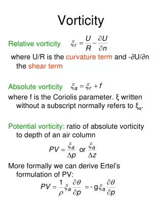
PV Analysis: Definitions • Basic Idea: • Potential vorticity represents the absolute vorticity an air column would have • if it were brought isentropically to a standard latitude and stretched/shrunk • to a standard depth • Analogous to “potential temperature” for an air parcel • Multiple Formulations: • Valid for Full Governing Equations • Equation [4.1] in Lackmann • Valid for Isentropic Analysis • Equation [4.2] in Lackmann • Valid for QG Analysis • Equation [2.38] in Lackmann • Valid for Shallow-water (Barotropic) Analysis • Equation [4.26] in Holton M. D. Eastin
PV Analysis: Synoptic-Scale Distribution • Basic Concepts: • Related to the product of absolute vorticity and static stability • Largest in polar regions (large f) and the stratosphere (large ∂θ/∂p) • Potential Vorticity Unit (PVU) → 10-6 K kg-1 m2 s-1 • → Troposphere PVU < 1.0 • → Stratosphere PVU > 2.0 • Dynamic Tropopause → Definition of the tropopause using a PV isosurface • → Often 1.5 or 2.0 PVU Dynamic Tropopause M. D. Eastin
PV Analysis: Synoptic-Scale Distribution • Basic Concepts: • PV Anomalies → Defined relative to a climatological average • Positive anomalies → Low pressure / Troughs • Negative anomalies → High pressure / Ridges • → Stratosphere is a “PV reservoir” • → Tropospheric synoptic-scale troughs are produced by “injections” • of stratospheric PV anomalies down into the troposphere Dynamic Tropopause M. D. Eastin
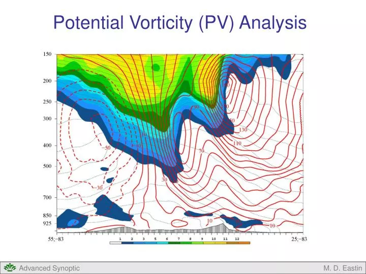
PV Analysis: Synoptic-Scale Distribution • Comparison to Isobaric Analyses: • Regions of low geopotential heights correspond to regions with large PV values • All troughs (even weak ones) show some evidence of PV > 1.5 (stratospheric air) • Cross-sections demonstrate the downward extrusion of large PV air associated • with each tropospheric trough 500mb Heights // 300-500mb PV PV // Potential Temperature N S N S M. D. Eastin
PV Analysis: Synoptic-Scale Distribution • Comparison to Isobaric Analyses: • Notice how locally strong geopotential height gradients (i.e., geostrophic jet maxima) • correspond to strong lateral gradients in stratospheric PV • This “double stair step” PV pattern is indicative of two distinct westerly jet maxima • [northern ↔ polar front jet southern ↔ subtropical jet] 500mb Heights // 300-500mb PV PV // Zonal winds N W E W S N S M. D. Eastin
PV Analysis: Synoptic-Scale Distribution • Dynamic Tropopause Maps: • A convenient way to plot the relevant features of all upper-air jet streams • Select a PV surface → usually 1.5 PVU or 2.0 PVU • Plot potential temperature, pressure, and winds on the PV surface • Provides a “topographic map” of the tropopause 500mb Heights // 300-500mb PV Potential Temperature and Winds on 2-PVU Surface M. D. Eastin
PV Analysis: Synoptic-Scale Distribution • Dynamic Tropopause Maps: • A convenient way to plot the relevant features of all upper-air jet streams • Select a PV surface → usually 1.5 PVU or 2.0 PVU • Plot potential temperature, pressure, and winds on the PV surface • Provides a “topographic map” of the tropopause 500mb Heights // 300-500mb PV Pressure and Winds on 2-PVU Surface M. D. Eastin
PV Analysis: Equations • Derivations and Interpretations: • The full derivations of the PV-conservation and PV-tendency equations for isentropic • coordinates are provided in the Lackmann text (Section 4.3.1) • PV-Conservation: • where • Valid for adiabatic, frictionless flow along isentropic surfaces • In such situations → PV remains constant, however, the relative vorticity, corioils • parameter, and/or static stability may change • → PV can be used as a “tracer” to track air parcel motions and • determine a parcels origin(s) at a previous time • → Evaluate non-conservative processes by documenting any • PV changes (which must have resulted from either • diabatic or frictional processes) ** Equation (4.16) in Lackmann text M. D. Eastin
PV Analysis: Equations • Derivations and Interpretations: • The full derivations of the PV-conservation and PV-tendency equations for isentropic • coordinates are provided in the Lackmann text (Section 4.3.1) • PV-Tendency: • where: and • Term A → Vertical Diabatic Forcing • → Relevant for vertically-stacked systems • Term B → Sheared Diabatic Forcing • → Relevant for vertically-tilted systems (developing cyclones / fronts) • Term C → Frictional Forcing (often neglected…we will too!!) Equation (4.17) in Lackmann text Term A Term B Term C M. D. Eastin
PV Analysis: Non-Conservation • How do Diabatic Processes change PV? Term A: Vertical Diabatic Forcing • Assume isentropic surfaces are horizontally-uniform (equivalent to geopotential height) • Heating maximum(due to condensation) is centered in the lower troposphere • Above heating max → local heights ascend → divergence • Below heating max → local isentropes / heights descend → convergence • As the height anomalies amplify, local height gradient accelerations will produce • convergence (divergence) below (above) the heating maximum (just like in QG theory…) • The heating maximum also alters the local static stability: • Above heating max → reduced static stability → PV decreases (-) • Below heating max → increased static stability → PV increases (+) M. D. Eastin
PV Analysis: Non-Conservation • How do Diabatic Processes change PV? Term B: Sheared Diabatic Forcing • Assume isentropic surfaces are tilted with height (as is often the case near fronts) • Heating maximum(due to condensation) is centered in the lower troposphere • In this case, the heating maximum alters the (1) local horizontal (isentropic) gradients, • (2) local static stability, and (3) local vertical shear (due to thermal wind balance), • producing a complex response, but… • Above heating max → PV always decreases (-) → horizontally displaced • Below heating max → PV always increases (+) → horizontally displaced • The magnitude and direction of horizontal displacement are functions of both • the vertical shear and the local heating rate M. D. Eastin
PV Analysis: Impermeability • Implications for Cases of Significant Mass Removal: • If we integrate the PV-conservation equation over an isentropic volume bounded laterally • by a streamline on which flow is adiabatic and frictionless, one can easy show • This is the “PV impermeability theorem” from Haynes and McIntyre (1987) • Powerful constraint as to how PV can change • PV is not “created” nor “destroyed, but rather “redistributed” • Any process that results in the significant movement of mass across an isentropic surface • will alter the local potential vorticity structure: • Heavy precipitation (thunderstorms and tropical cyclones) • Dry deposition of large particles (sand storms) Equation (4.24) in Lackmann text M. D. Eastin
PV Analysis: Inversion • Invertibility Principle: • Allows the user to “recover” the balanced wind and thermodynamic fields associated with • any given PV anomaly • The balanced flow (red) and related temperature and pressure structures (not shown) • extend to spatial locations far removed from that of the anomaly itself (green) • Analogous to the far electric fields associated with point charges • (…this is one reason why you are required to take Physics-2) M. D. Eastin
PV Analysis: Inversion • Invertibility Principle: • Allows the user to “recover” the balanced wind and thermodynamic fields associated with • any given PV anomaly • The PV field can be sub-divided into as many “PV pieces” as desired • Each PV piece can then be inverted separately (called “piecewise inversion”) • to determine its partial contribution to the total structure of a given system • You could also explore partial • contributions from different • atmospheric constituents: • water vapor • ozone • pollution 1 3 2 M. D. Eastin
PV Analysis: Advantages / Disadvantages • Advantages: • Synoptic-scale dynamic tropopause mapsallows one to easily see all • relevant upper-level jet streaks and system structure on one map • Through piecewise inversion, one can diagnose which physical processes • were responsible for the “observed” PV distribution. • Post-event analysis of poorly forecast cases • Evaluate and quantify contributions from non-conservative processes • Evaluate and quantify numerical model errors in system structure • Learn limitations of numerical models in certain forecast situations • Allows forecasters to assign confidence to each numerical model • (see examples on next few slides…) • Disadvantages: • Computations must be performed to interpolate pressure, wind, and • moisture data onto isentropic surfaces • Nearly impossibleto conduct piecewise inversion from only observations • (must use numerical model analysis and forecast fields**) M. D. Eastin
PV Analysis: Advantages / Disadvantages Diagnosing contributions to System Structure: Potential Temperature (5-K interval) // PV (1-PVU interval) Extra-tropical cyclone Large deep stratospheric source Smaller low-level diabatic source Tropical cyclone Minimal stratospheric source Large low-level diabatic source Sub-tropical (hybrid) cyclone Some stratospheric source Equal low-level diabatic source M. D. Eastin
PV Analysis: Advantages / Disadvantages • Diagnosing contributions to Model Error: • January 2000 snowstorm across the Southeast • One model (RUC) provided good forecasts • Other popular models (AVN/GFS and NAM/Eta) • did NOT forecast the event well…Why? • Underestimated diabatic PV production • from two regions of heavy precipitation • which eventually merged over SC • Human forecasters could see the errors RUC Analysis SLP // 900-700mb PV Radar // 24-hr Eta precipitation forecast Eta 24-hr SLP // 900-700mb PV M. D. Eastin
PV Analysis: Websites • Real-time and Archived Analyses: • SUNY Albany: http://www.atmos.albany.edu/index.php?d=wx_data • University of Reading: http://www.met.reading.ac.uk/Data/CurrentWeather/ • MIT: http://wind.mit.edu/~reanal/pv.html • University of Washington: http://www.atmos.washington.edu/~hakim/tropo/info.html • (personal webpage) • University of Oklahoma: http://weather.ou.edu/~scavallo/real_time_plots.html • (personal webpage) M. D. Eastin
References Bishop, C. H. and A. J. Thorpe, 1994: Potential vorticity and the electrostatics analogy: Quasi-geostrophic theory. Quarterly Journal of the Royal Meteorological Society, 120, 713-731. Bluestein, H. B, 1993: Synoptic-Dynamic Meteorology in Midlatitudes. Volume I: Principles of Kinematics and Dynamics. Oxford University Press, New York, 431 pp. Bluestein, H. B, 1993: Synoptic-Dynamic Meteorology in Midlatitudes. Volume II: Observations and Theory of Weather Systems. Oxford University Press, New York, 594 pp. Brennan, M. J., G. M. Lackmann, and K. A. Mahoney, 2008: Potential vorticity (PV) thinking in operations: The utility of non-conservation. Weather and Forecasting, 23, 168-182 Davis, C. A., 1992b: Piecewise potential vorticity inversion. Journal of Atmospheric Science, 49, 1397-1411 Eliassen A., and E. Kleinschmidt, 1957: Dynamic Meteorology, Encyclopedia of Physics, Springer Publishing, 1-154 Haynes, P. H., and M. E. McIntyre, 1987: On the evolution of vorticity and potential vorticity in the presence of diabatic heating and frictional or other forces. Journal of Atmospheric Science, 44, 828-841 Hoskins, B.J., McIntyre, M.E. and Robertson, A.W., 1985: On the use and significance of isentropic potential vorticity maps. Quarterly Journal of the Royal Meteorological Society, 111, 877-946. Lackmann, G., 2011: Mid-latitude Synoptic Meteorology – Dynamics, Analysis and Forecasting, AMS, 343 pp. Rossby, C. G., 1940: Planetary flow patterns in the atmosphere. Quarterly Journal of the Royal Meteorological Society, 66, 68-87. Samuelson, R. M., 2003: Rossby, Ertel, and potential vorticity. University of Princeton, 9 pp. Schubert W., and co-authors, 2004: English translations of twenty-one of Ertel’s papers on geophysical fluid dynamics, MeteorologischeZeitschrift, 13, 527-576. M. D. Eastin