Download
1 / 20
200 likes | 314 Views
LLNL AS3 Seminar Nov 10, 2010. Caldwell, Peter, 2010: California Wintertime Precipitation Bias in Regional and Global Climate Models. J. Appl. Meteor. Climatol ., 49, 2147–2158.doi: 10.1175/2010JAMC2388.1. UCRL: LLNL-PRES-413982. Background:. Why are rainfall changes important?

E N D
LLNL AS3 Seminar Nov 10, 2010 Caldwell, Peter, 2010: California Wintertime Precipitation Bias in Regional and Global Climate Models. J. Appl. Meteor. Climatol., 49, 2147–2158.doi: 10.1175/2010JAMC2388.1 Prepared by LLNL under Contract DE-AC52-07NA237344. UCRL: LLNL-PRES-413982
Background: • Why are rainfall changes important? • increases=floods, • decreases=droughts. • Why is precipitation modeling important? • models are our main way of predicting climate change.
Background: • Why is modeling precipitation hard? • precipitation depends in a complicated way on small-scale processes. Interaction between microphysical processes in a typical atmospheric model. Adapted from Houze (1993) • How can we make progress? • higher resolution means less parameterization dependence. • biggest difference expected in • mountainous areas. Annual-average precip patterns follow topography, which is more realistic at higher resolution.
Motivation: WRF CCSM3 UW (Obs) NOAA (Obs) Results for one 12 km res RCM: • RCM substantially overestimated wintertime precipitation. • Regional averages from RCM showed no clear improvement over its driving GCM. 1-σ bounds from monthly data Seasonal cycle of precip averaged over the CA coast and mountain regions. WRF=40 yr run forced by a1°x1.25°CCSM3 simulation.
Motivation: We’re Not Alone… RCM papers with West Coast overprediction: • Giorgi et al. (J. Clim, 1994) • Kim et al. (J. Hydromet., 2000) • Pan et al. (JGR, 2001) • Snyder et al. (GRL, 2002) • Kim and Lee (J. Hydromet, 2003) • Bell et al. (J. Clim., 2004) • Han and Roads (Clim. Change, 2004) • Liang et al. (J. Clim.,2004) • Salathe et al. (J. Clim., 2008) • Leung et al. (J. Clim, 2003), 2 RCMs • Duffy et al. (J. Clim., 2006) , 4 RCMs Seasonal cycle of present-day P averaged over the Western US. Red = RCM, green = driving GCM (not always available), blue and black = obs. From Duffy et al (2006, J. Clim) Until now, evaluation of RCM precipitation biases has been anecdotal and disorganized…
Methodology: Data Sets Compare precip from obs, RCMs, and GCMs simulations for Nov-Mar of 1981-1998: • RCMs: • 6 models from the North American Regional Climate Change Assessment Program (NARCCAP, narccap.ucar.edu). • Forced from National Center for Environmental Prediction Reanalysis II (NCEP2). • Run at 50 km grid spacing over continental US. • GCMs: • 13 models from the Coupled Model Intercomparison Project 3 experiment (www-pcmdi.llnl.gov/ • ipcc/about_ipcc.php, CMIP3). • 1 global model (GFDL Hi) from NARCCAP. • Atmosphere-only runs: forced by observed SST and 20th century greenhouse gases. • Gridded Observations: • Gauge Data: • UW: www.hydro.washington.edu/ • Lettenmaier/Data/gridded/ • index_hamlet.html • Unified: www.cdc.noaa.gov/cdc/ • data.unified.html • CRU: www.cru.uea.ac.uk/~timm/ • grid/CRU_TS_2_1.html • UDel: www.cdc.noaa.gov/data/gridded/data.Udel_AirT_Precip.html • Gauge/Satellite/Radar Data: • CMAP: www.cdc.noaa.gov/data/ • gridded/data.cmap.html • GPCP:www.gewex.org/gpcp.html
Methodology: Averaging Guiding question:does resolution improve simulation? • Previous studies use metrics which reward higher output resolution independent of whether physics is improved. • Benefits of CA average: • fair comparison across resolution • reduces dimensionality for easy analysis • increases statistical robustness. CCSM3 WRF DJF Average Precip Climatology (mm day-1) 0.8 2.4 4 5.6 7.2 8.810.4 12 A metric that makes higher resolution models look better.
Methodology: Averaging Simple Bilinear • How to take averages? 4 methods are considered; agreement is used as a measure of uncertainty. Landmask/Conservative Conservative Averaging methods applied to CNRM (2.8o) model.
Averaging Strategy Validation Model Resolution (degrees) • Averaging error typically <10% for dx<3°. • Inconsistent land-frac → trouble for Land-mask method (here-after omitted). • Bilinear is ok, but Conservative is always slightly better. • Simple method does surprisingly well. • Except Simple, methods under-predict average. 2.80 2.26 2.80 2.80 2.80 3.14 1.12 1.40 1.56 1.87 4.50 4.50 Difference between CA average on native grid vs after conservatively regridding to each GCM grid and applying the 4 averaging techniques. “+” means the method overpredicted the true average.
Results: Precip Bias • Using UW or CRU as “truth” (instead of Unified) would yield similar results. Using CMAP or GPCP would underpredict. • GCMs often too dry. • Previous studies (based on CMAP, GPCP) suggested GCMs were too wet… • is this an AMIP/CMIP difference? Bias in Nov-Mar CA-average precip (model – Unified obs) for each model. Errorbars = t-statistic 95% confidence intervals. Different colored errorbars indicate different averaging techniques. Dots= ensemble members.
Results: Precip Bias • All RCMs except HadRM3 are significantly too wet. • In general, resolution is not a good indicator of model skill. • Poor resolution isn’t the leading source of model error! • Is improvement being masked by GCM tuning? Bias in Nov-Mar CA-average precip (model – Unified obs) for each model. Errorbars = t-statistic 95% confidence intervals. Different colored errorbars indicate different averaging techniques. Dots= ensemble members.
Interpretation: Is High-Res Worth It? • May work better in other regions. • High resolution still needed for studies which require fine-scale output not available from traditional GCMs (see below). CCSM3 WRF Obs (University of WA) Precipclima-tology from Caldwell et al (Climatic Change, ‘09) DJF Average Precip Climatology (mm day-1) 0.8 2.4 4 5.6 7.2 8.810.4 12
Results:Exceedence Probabilities • GCM results have no consistent bias. • Expectation was excessive weak events? • GFDL Hi behaves like RCMs. • Resolution is not a good predictor of model behavior. Obs RCMs Re GCMs Colors = percent of the time it is raining harder than the given threshold (on left y axis). Blue line = percent of the time it is raining harder than 0.1mm/day (scale on right-hand y axis).
Results:Exceedence Probabilities • Except CRCM, all RCMs overpredict strong events. • RCM precip frequency (blue line) tends to be low. • RCM over-prediction is due to overly strong heavy events? Obs RCMs Re GCMs Colors = percent of the time it is raining harder than the given threshold (on left y axis). Blue line = percent of the time it is raining harder than 0.1mm/day (scale on right-hand y axis).
Heavy-Event Bias Verification • Overpredicted CA-average extremes could be due to overpredictedarea of heavy precip instead of intensity. • Tested by computing the fraction of models over-predicting when conservatively regridded to NOAA Unified obs. • overpredictionis due to intensity. Fraction of models (RCMs on left, GCMs on right) overpredictingprecip frequency (top) or 99% magnitude (bottom). Overprediction determined by regridding to, then comparing against Unified.
Interpretation: Sources of Bias • Consistency of high resolution model bias suggests bias is due to a conceptual flaw rather than the intricacies of a particular code (which is good). • The fact that bias comes from overpredicted intensity of major storms means that case studies of individual events can be used to explore the problem. Precip (mm day-1) Chin, Hung-Neng S., Peter M. Caldwell, David C. Bader, 2010: Preliminary Study of California Wintertime Model Wet Bias. Mon. Wea. Rev., 138, 3556–3571. For individual storms, Increasing resolution increases precip Models tend to overpredict regardless of microphysics scheme Choice of observational dataset important 12/30/96 3/7/95 3/6/89 12/10/95 Pineapple El Nino La Nina Synoptic Express Cyclone Precip rates for 4 storms simulated by WRF with different microphysics schemes and resolution.
Results: Variability • The best RCMs have reasonable variance. Others are too high. • GCM variance is too low (consistent with previous studies) Standard deviation of daily or wintertime average (blue) precip from each model. Daily values for models without daily data are mapped to zero.
Conclusions: • CA averages can be robustly determined for dx<3° • Conservative averaging best, but bilinear, simple ok. • RCMs systematically overestimate CA wintertime precip • Due to excessive strong events (be wary of flooding studies!) • Supports use of individual storms to test/improve models • Variance bias scales with magnitude • GCMs tend to underestimate CA wintertime precip • Previous studies used GPCP and CMAP, which underpredict • Bias isn’t correlated to resolution… other factors dominate • GCM variability isunderpredicted
Conclusions: • RCMs offer little improvement in CA average • RCM deficiencies counteract benefits of increased resolution • Value is added at scales unresolved by GCMs • This result could change for other variables (e.g. snowpack) Goals should be carefully considered in deciding whether to downscale.