Download
1 / 33
350 likes | 425 Views
Learn the parametrization using slope angle, Lagrange multipliers, and analytical solutions for the Brachistochrone problem with non-conservative velocity-dependent frictional force. Explore the constraints and natural boundary conditions involved.

E N D
Brachistochrone Under Air Resistance Christine Lind 2/26/05 SPCVC
Brachistochrone Setup: • Initial Point P(x0,y0) • Final Point Q(x1,y1) • Resistance Force Fr • Slope Angle
Geometric Constraints • Parametric Approach: • Start by using arclength (s) as the parameter • Parametrized by arclength: (curves parametrized by arclength have unit speed)
Energy Constraint? • Normally we use conservation of energy to solve for velocity in terms of the other variables • We have a Non-Conservative system, so what do we do?
Energy Constraint? • Energy is lost to work done by the resistance force:
Energy Constraint • Non-conservative system: • Constraint parametrized by time: • Constraint parametrized by arclength:
Problem Formulation: • Boundary & Initial Conditions: • Minimize the time integral: • Other constraints: How do we incorporate them?
Lagrange Multipliers • Introduce multipliers, vector: • Create modified functional: where
Euler-Lagrange Equations • System of E-L equations: • Additional boundary conditions:
Note: Note: Additional Constraints Appear as E-L equations! 7 Euler-Lagrange Equations:
Natural Boundary Conditions: Note: v1 is not necessarily zero, so:
Note: (s),(s) constants (s)=((s)) Lagrange Multipliers - Solved! • Using: • Determine the Lagrange Multipliers:
First Integral • Recall: No explicit s-dependence! • First Integral:
Still need constraints... Parametrize by Slope Angle • Define f() to be the inverse function of (s): • f() continuously differentiable, monotonic • Now we minimize:
Modified Functional • Transform modified problem in terms of :
First Integral! (Old Equations) 7 Euler-Lagrange Equations
Solve for v() • Using Lagrange Multipliers and First Integral: • Obtain:
Solve for Initial Angle 0 • Evaluate at 0: • Obtain Implicit Equation for initial slope angle:
Solving for f() • Rearrange E-L equation: • Obtain ODE: ( Recall that we already have v(), 0, & initial condition f(0) = 0 )
Solving for x() and y() • Integrate the E-L equations • Obtain
Seems like we are done... • What about parameters 1 & v1? Appear everywhere, due to: • How can we solve for them?
Newton’s Method... • Use the equations for x() and y() and the corresponding boundary conditions: • Now we really are done!
0 = /2 Example: Air Resistance • Take R(v) = k v (k - coefficient of viscous friction) • Newtonian fluid • first order approx. for air resistance • Let x0 = 0, y0 = 0, v0 = 0,
Solve for v() Quadratic Formula: ( take the negative root to satisfy v(0) = 0 )
(Straight Line) (Cycloid) Results:
Conclusions • Different approach to the Brachistochrone • parametrization by the slope angle • use of Lagrange Multipliers • Gained: • analytical solution for non-conservative velocity-dependent frictional force • Lost ( due to definition s = f() ): • ability to descibe free-fall and cyclic motion