Download
1 / 61
610 likes | 635 Views
Explore methods to estimate demographic parameters from DNA data, focusing on African populations with a composite-likelihood approach. Understand ancient population structures and migration patterns using statistical genetics.

E N D
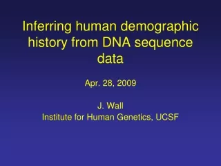
Inferring human demographic history from DNA sequence data Apr. 28, 2009 J. Wall Institute for Human Genetics, UCSF
Standard model of human evolution(Origin and spread of genus Homo) 2 – 2.5 Mya
Standard model of human evolution(Origin and spread of genus Homo) ? ? 1.6 – 1.8 Mya
Standard model of human evolution(Origin and spread of genus Homo) 0.8 – 1.0 Mya
Standard model of human evolutionOrigin and spread of ‘modern’ humans 150 – 200 Kya
Standard model of human evolutionOrigin and spread of ‘modern’ humans ~ 100 Kya
Standard model of human evolutionOrigin and spread of ‘modern’ humans 40 – 60 Kya
Standard model of human evolutionOrigin and spread of ‘modern’ humans 15 – 30 Kya
Estimating demographic parameters • How can we quantify this qualitative scenario into an explicit model? • How can we choose a model that is both biologically feasible as well as computationally tractable? • How do we estimate parameters and quantify uncertainty in parameter estimates?
Estimating demographic parameters • Calculating full likelihoods (under realistic models including recombination) is computationally infeasible • So, compromises need to be made if one is interested in parameter estimation
African populations 10 populations 229 individuals
African populations Mandenka (bantu) 61 autosomal loci ~ 350 Kb sequence data Biaka (pygmies) San (bushmen)
A simple model of African population history T g1 m g2 Biaka (or San) Mandenka
Estimation method We use a composite-likelihood method (cf. Plagnol and Wall 2006) that uses information from the joint frequency spectrum such as: Numbers of segregating sites Numbers of shared and fixed differences Tajima’s D FST Fu and Li’s D*
Estimation method We use a composite-likelihood method (cf. Plagnol and Wall 2006) that uses information from the joint frequency spectrum such as: Numbers of segregating sites Numbers of shared and fixed differences Tajima’s D FST Fu and Li’s D*
Estimating likelihoods Pop1 Pop2
Estimating likelihoods Pop 1 private polymorphisms Pop1 Pop2
Estimating likelihoods Pop 1 private polymorphisms Pop 2 private polymorphisms Pop1 Pop2
Estimating likelihoods Pop 1 private polymorphisms Pop 2 private polymorphisms Shared polymorphisms Pop1 Pop2
Estimation method We use a composite-likelihood method (cf. Plagnol and Wall 2006) that uses information from the joint frequency spectrum such as: Numbers of segregating sites Numbers of shared and fixed differences Tajima’s D FST Fu and Li’s D*
Estimating likelihoods We assume these other statistics are multivariate normal. Then, we run simulations to estimate the means and the covariance matrix. This accounts (in a crude way) for dependencies across different summary statistics.
Composite likelihood We form a composite likelihood by assuming these two classes of summary statistics are independent from each other We estimate the (composite)-likelihood over a grid of values of g1, g2, T and M and tabulate the MLE. We also use standard asymptotic assumptions to estimate confidence intervals
Estimates (with 95% CI’s) Parameter Man-Bia Man-San g1 (000’s)0 (0 – 3.8) 0 (0 – 3.8) g2 (000’s)4 (0 – 7.9) 2 (0 – 11) T(000’s) 450 (300 – 640) 100 (77 – 550) M (= 4Nm) 10 (8.4 – 12) 3 (2.2 – 4)
Fit of the null model How well does the demographic null model fit the patterns of genetic variation found in the actual data?
Fit of the null model How well does the demographic null model fit the patterns of genetic variation found in the actual data? Quite well. The model accurately reproduces both parameters used in the original fitting (e.g., Tajima’s D in each population) as well as other aspects of the data (e.g., estimates of ρ = 4Nr)
Estimates (with 95% CI’s) Parameter Man-Bia Man-San g1 (000’s)0 (0 – 3.8) 0 (0 – 3.8) g2 (000’s)4 (0 – 7.9) 2 (0 – 11) T(000’s) 450 (300 – 640) 100 (77 – 550) M (= 4Nm) 10 (8.4 – 12) 3 (2.2 – 4)
Population growth population size time
Population growth population size time spread of agriculture and animal husbandry?
Estimates (with 95% CI’s) Parameter Man-Bia Man-San g1 (000’s)0 (0 – 3.8) 0 (0 – 3.8) g2 (000’s)4 (0 – 7.9) 2 (0 – 11) T(000’s) 450 (300 – 640) 100 (77 – 550) M (= 4Nm) 10 (8.4 – 12) 3 (2.2 – 4)
Ancestral structure in Africa At face value, these results suggest that population structure within Africa is old, and predates the migration of modern humans out of Africa. Is there any evidence for additional (unknown) ancient population structure within Africa?
Model of ancestral structure Archaic human population T g1 m g2 Biaka (or San) Mandenka
Standard model of human evolutionOrigin and spread of ‘modern’ humans ~ 100 Kya
Admixture mapping Modern human DNA Neandertal DNA
Admixture mapping Modern human DNA Neandertal DNA
Admixture mapping Modern human DNA Neandertal DNA
Admixture mapping Modern human DNA Neandertal DNA
Admixture mapping Modern human DNA Neandertal DNA Orange chunks are ~10 – 100 Kb in length
Genealogy with archaic ancestry time Modern humans Archaic humans present
Genealogy without archaic ancestry time Modern humans Archaic humans present
Our main questions • What pattern does archaic ancestry produce in DNA sequence polymorphism data (from extant humans)? • How can we use data to • estimate the contribution of archaic humans to the modern gene pool (c)? • test whether c > 0?
Genealogy with archaic ancestry(Mutations added) time Modern humans Archaic humans present
Genealogy with archaic ancestry(Mutations added) time Modern humans Archaic humans present
Patterns in DNA sequence data Sequence 1 A T C C A C A G C T G Sequence 2 A G C C A C G G C T G Sequence 3 T G C G G T A A C C T Sequence 4 A G C C A C A G C T G Sequence 5 T G T G G T A A C C T Sequence 6 A G C C A T A G A T G Sequence 7 A G C C A T A G A T G
Patterns in DNA sequence data Sequence 1 A T C C A C A G C T G Sequence 2 A G C C A C G G C T G Sequence 3 T G C G G T A A C C T Sequence 4 A G C C A C A G C T G Sequence 5 T G T G G T A A C C T Sequence 6 A G C C A T A G A T G Sequence 7 A G C C A T A G A T G
Patterns in DNA sequence data Sequence 1 A T C C A C A G C T G Sequence 2 A G C C A C G G C T G Sequence 3 T G C G G T A A C C T Sequence 4 A G C C A C A G C T G Sequence 5 T G T G G T A A C C T Sequence 6 A G C C A T A G A T G Sequence 7 A G C C A T A G A T G We call the sites in red congruent sites – these are sites inferred to be on the same branch of an unrooted tree
Linkage disequilibrium (LD) LD is the nonrandom association of alleles at different sites. Low LD: AC High LD: A C A T A C ACA C A T A C G C G T G T G T G C G T G T G T High recombination Low recombination
Measuring ‘congruence’ To measure the level of ‘congruence’ in SNP data from larger regions we define a score function S* = where S (i1, . . . ik) = and S (ij, ij+1) is a function of both congruence (or near congruence) and physical distance between ij and ij+1.