Download
1 / 25
250 likes | 269 Views
This article discusses the digitization of analogue filters using the Bilinear Transform technique, including its advantages and disadvantages. It also explores filter implementation methods, such as Direct Form I and II, and the CSOS structure.

E N D
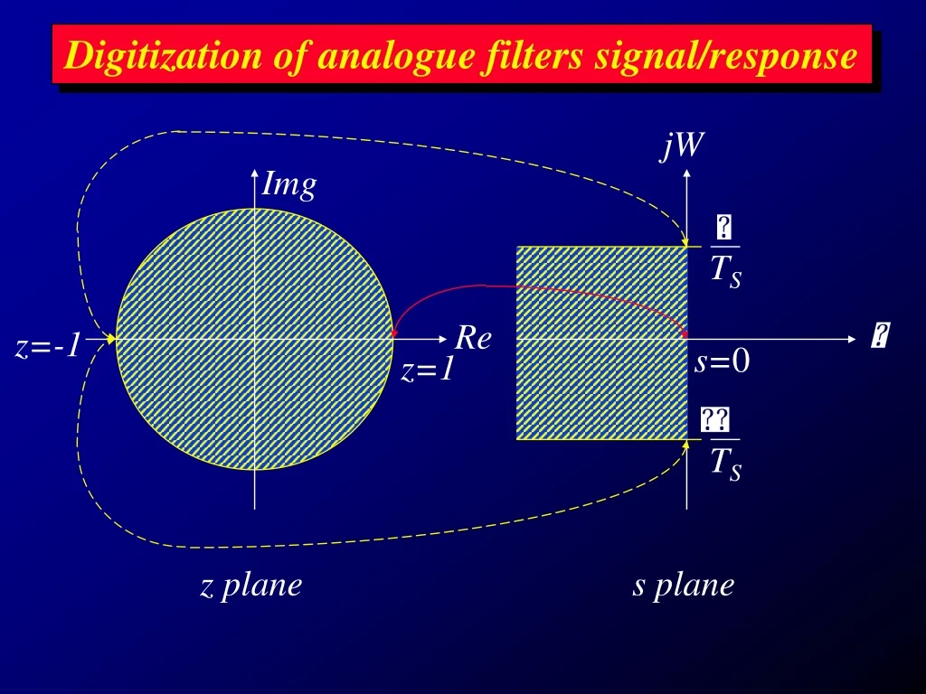
TS Digitization of analogue filters signal/response jW Img Re z=-1 s=0 z=1 TS z plane s plane
are mapped to nowhere, Frequencies beyond Digitization of analogue filters signal/response Disadvantage of the Pole Mapping technique leading to aliasing error Bilinear Transform A nonlinear one-to-one mapping from the j axis of the s-plane to the unit circle in the z plane
Bilinear Transform
Bilinear Transform is mapped to The left half s plane is mapped onto the inside of the unit circle in the z plane The stability of a system is preserved in the transform
Bilinear Transform With z = ejand s = j, we have For small value of
Pole Mapping in Bilinear Transform Consider a pole at s = spis mapped to a pole at
Bilinear Transform TABLE I f 4fs 0.95 2fs 0.90 f fs 0.80 fs/2 0.64 fs = 1/TS fs/4 0.42 fs/8 0.24 fs/16 0.12 0 0
Bilinear Transform TABLE I f 4fs 0.95 1.1 2fs 0.90 1.2 fs 0.80 1.3 fs/2 0.64 1.5 fs/4 0.42 1.8 fs/8 0.24 2.0 fs/16 0.12 0 0
Bilinear Transform The conversion listed Table I is not realistic Consider the sampling lattice in the frequency domain for N = 16 fs 2fs 3fs 4fs 5fs 6fs 7fs fs 7fs 6fs 5fs 4fs 3fs 2fs fs 0 0 16 16 16 16 16 16 16 2 16 16 16 16 16 16 16 Even for low analogue frequencies, the accuracy of mapping from to is not uniform
Bilinear Transform The conversion listed Table I is not realistic Consider the sampling lattice in the frequency domain for N = 16 fs 2fs 3fs 4fs 5fs 6fs 7fs fs 7fs 6fs 5fs 4fs 3fs 2fs fs 0 0 16 16 16 16 16 16 16 2 16 16 16 16 16 16 16 is wasted as the input signal cannot reach beyond fs/2 after sampling
Frequency Prewarping The behaviour of bilinear transform is nonlinear and can be compensated with frequency prewarping
Frequency Prewarping The behaviour of bilinear transform is nonlinear and can be compensated with frequency prewarping
Frequency Prewarping TABLE II f * fs 0 2.0 fs/2 2.0 fs/4 0.32fs 2.0 fs/8 0.13fs 2.0 fs/16 0.06fs 0 0 0
Frequency Prewarping The conversion listed Table II Consider the sampling lattice in the frequency domain for N = 16 fs 2fs 3fs 4fs 5fs 6fs 7fs fs 7fs 6fs 5fs 4fs 3fs 2fs fs 0 0 16 16 16 16 16 16 16 2 16 16 16 16 16 16 16 Even for low analogue frequencies, the accuracy of mapping from to is not uniform
Filter Implementation - Direct Form I NF M bk z-kx(n) y(n)= ak z-ky(n) + k= -NF k=1 b-NF z x(n) y(n) b0 + + z-1 z-1 a1 bNF z-1 aM
Filter Implementation - Direct Form II NF M bk z-kx(n) y(n)= ak z-ky(n) + k= -NF k=1 LET , then
Filter Implementation - Direct Form II Filter Implementation - Direct Form II
Filter Implementation - Direct Form II + x(n) u(n) z-1 a1 z-1 aM
Filter Implementation - Direct Form II b-NF z u(n) y(n) b0 + z-1 bNF
b-NF z y(n) u(n) b0 + z-1 bNF Filter Implementation - Direct Form II x(n) + z-1 a1 z-1 aM Canonical structure - minimum number of delays
Filter Implementation - CSOS CSOS - Cascade Combination of Second-Order Sections
Filter Implementation - CSOS Template