4.3 Verification of successful prediction

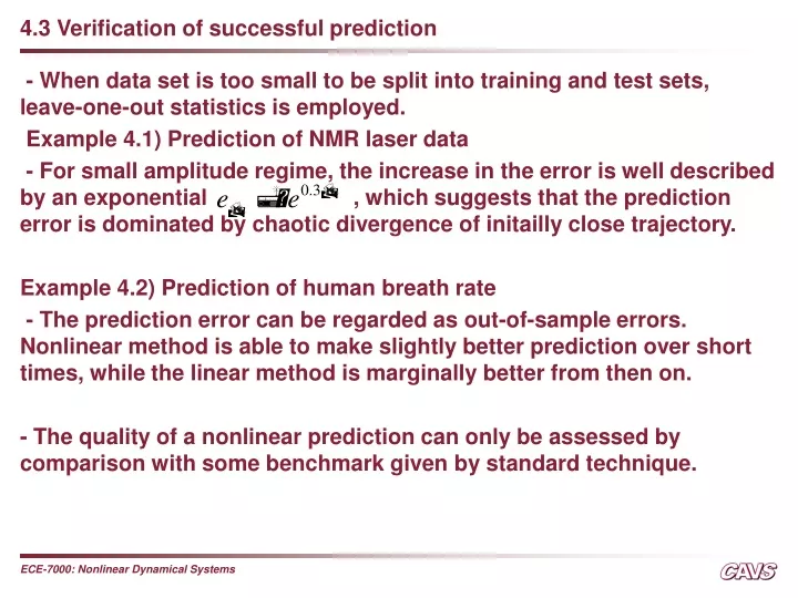
1. 4.3 Verification of successful prediction • - When data set is too small to be split into training and test sets, leave-one-out statistics is employed. • Example 4.1) Prediction of NMR laser data • - For small amplitude regime, the increase in the error is well described by an exponential , which suggests that the prediction error is dominated by chaotic divergence of initailly close trajectory. • Example 4.2) Prediction of human breath rate • - The prediction error can be regarded as out-of-sample errors. Nonlinear method is able to make slightly better prediction over short times, while the linear method is marginally better from then on. • - The quality of a nonlinear prediction can only be assessed by comparison with some benchmark given by standard technique.

2. 4.4 Cross-prediction errors: probing stationarity • - In a system where different dynamics are at work, • - Break the available data into Segments which is long enough to • make simple nonlinear predictions. • - Two segments and , compute rms prediction error using • as the training set but use as the test set. • - The cross-prediction error as a funtion of i and j reveals which • segments differ in their dynamics. • Example 4.3) Non-stationarity of breath rate • - Split the recording into 34 non-overlapping segment of 1000 • points (500 s) each. • - use unit delay and three dimentional embeddings. • - Segments from the first half are useless for prediction in the second • half, and vice versa. • - What statistic to use?

3. 4.5 Simple nonlinear noise reduction • - Noise reduction means that one tries to decompose every signal time • series value into two component, signal and random fluctuations. • - Assume the data can thought of as an additive superposition of two • different components. • - Power spectrum is a tool for this distinction • - Random noise has a flat or broad spectrum, whereas periodic • signals have sharp spectral lines. • - This approach fails for deterministic chaotic dynamics •  output of such system leads to broad band spectra itself and thus • possesses spectral properties generally attributed to random • noise. • - Deterministic structure will closely follow what we have done for • nonlinear predictions.

4. 4.5 Simple nonlinear noise reduction • - , • is random noise with at least fast decaying autocorrelations and • no correlation with the signal , and • - How can we recover the signal , • given only the noise sequence ? • - Throw away measurements and replace them by a prediction • - Revise time and predict the desired value from the subsequent • measurements. • - The above two fails to recover signal • - Solve the implicit relation

5. 4.5 Simple nonlinear noise reduction • - In order to obtain estimate for the value of , • we form delay vector and determine those • which are close to . • - The average value of is then used as a cleaned value • - No matter how small a value of we choose, is never empty • - If we choose too small, the worst thing that can happen is that the • only neighbour found is itself. • - However, yields the estimate , which just means that • no correction is made at all.

6. 4.5 Simple nonlinear noise reduction • - Due to the assumed independence of signal and noise, • - How we make sure that all we do is to reduce noise without distorting • the signal? • - The error due to distortion must be considerably smaller than the • noise amplitude.