On Map-Matching Vehicle Tracking Data

1. On Map-Matching Vehicle Tracking Data Sotiris Brakatsoulas Dieter Pfoser {sbrakats|pfoser}@cti.gr Carola Wenk Randall Salas {wenk|rsalas}@cs.utsa.edu

2. Motivation • Moving Objects Data • Vehicle Tracking Data • Trajectories

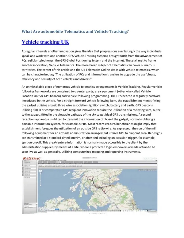
3. Motivation • Use of Floating Car Data (FCD)generated by vehicle fleet as samples to assess to overall traffic conditions • Floating car data (FCD) • basic vehicle telemetry, e.g., speed, direction, ABS use • the position of the vehicle ( tracking data) obtained by GPS tracking • Traffic assessment • data from one vehicle as a sample to assess to overall traffic conditions – cork swimming in the river • large amounts of tracking data(e.g., taxis, public transport, utility vehicles, private vehicles)  accurate picture of the traffic conditions

4. Traffic Condition Parameters • Travel times • Traffic count Relating tracking data to road network  Map-Matching

5. Outline • Vehicle Tracking Data, Trajectories • errors in the data • Incremental MM Technique • “classical” approach • Global MM Technique • curve – graph matching • Quality of the Map-Matching • Measures • Empirical Evaluation • Conclusions and future work

6. Vehicle Tracking Data • Sampling the movement • Sequence (temporal) of GPS points • affected by precision of GPS positioning error • measurement error • Interpolating position samples  trajectory • affected by frequency of position samples • sampling error

7. P2 P1 Vehicle Tracking Data • Error example • vehicle speed 50km/h (max) • sampling rate 30s 208m • Map-matching • matching trajectories to a path in the road network 417m

8. Map Matching • Perception of the problem • online vs. offline map-matching • Incremental method • incremental match of GPS points to road network edges • classical approach • Global method • matching a curve to a graph • finding similar curve in graph

9. Position-by-position, edge-by-edge strategy to map-matching α i,1 α i,3 c 1 d c d 3 3 1 p l p i d i i-1 2 c 2 α i,2 Incremental Method

10. c 1 c 3 pi c 2 pi+1 pi-1 Incremental Method • Introducing globality • Look-ahead to evaluate quality of different paths • to match one edge consider its consequences • Example: depth = 2 (depth = 1  no look-ahead)

11. Incremental Method • Actual map-matching • evaluates for each trajectory edges (GPS point) a finite number of edges of the road network graph • O(n) (n – trajectory edges) • Initialization done using spatial range query • Map-matching dominates initialization cost

12. Global Method • Try to find a curve in the road network (modeled as a graph embedded in the plane with straight-line edges) that is as close as possible to the vehicle trajectory • Curves are compared using • Fréchet distance and • Weak Fréchet distance • Minimize over all possible curves in the road network

13. Fréchet Distance • Dog walking example • Person is walking his dog (person on one curve and the dog on other) • Allowed to control their speeds but not allowed to go backwards! • Fréchet distance of the curves: minimal leash length necessary for both to walk the curves from beginning to end

14. Fréchet Distance • Fréchet Distance • where α and β range over continuous non-decreasing reparametrizations only • Weak Fréchet Distance • drop the non-decreasing requirement for α and β • Well-suited for the comparison of trajectories since they take the continuity of the curves into account

15. Free Space Diagram • Decision variant of the global map-matching problem • for a fixed ε > 0 decidewhether there exists a path in the road network withdistance at most ε to the vehicle trajectory α • For each edge (i,j) ina graphG let its corresponding Freespace Diagram FDi,j = FD(α, (i,j)) i α (i,j) (i,j) 1 0 ε 1 2 3 4 5 6 α j

16. Free Space Surface • Glue free space diagrams FDi,j together according to adjacency information in the graph G • Free space surface of trajectory α and the graph G G α shown implicitely by the free space surface

17. Free Space Surface • TASK: Find monotone path in free space surface • starting in some lower left corner, and • ending in some upper right corner G

18. Free Space Surface • Sweep-line algorithm • maintain points on sweep line that are reachable by some monotone path in the free space from some lower-left corner • updating reachability information Dijkstra style • Minimization problem for ε is solved using parametric search or binary search • Parametric search (binary search) • O(mn log2(mn)) time(m – graph edges, n – trajectory edges) • Weak Fréchet distance, drop monotone requirement • O(mn log mn) time

19. Quality of Matching Result • Comparing Fréchet distance of original and matched trajectory • Fréchet distances strongly affected by outliers, since they take the maximum over a set of distances. • How to fix it? Replace the maximum with a path integral over the reparametrization curve (α(t),β(t)): • Remark: Dividing by the arclength of the reparametrization curve yields a normalization, and hence an „average“ of all distances.

20. Quality of Matching Result • Unfortunate drawbacks • we do not know how to compute this integral. • Approximate integral by sampling the curves and computing a sum instead of an integral. • 2m • very costly and gives no approximation guarantee or convergence rate

21. Empirical Evaluation • GPS vehicle tracking data • 45 trajectories (~4200 GPS points) • sampling rate 30 seconds • Road network data • vector map of Athens, Greece(10 x 10km) • Evaluating matching quality • results from incremental vs. global method • Fréchet distance vs. averaged Fréchet distance (worst-case vs. average measure)

22. Empirical Evaluation • Fréchet vs. Weak Fréchet distance produces same matching result • no backing-up on trajectories (course sampling rate) or • road network (on edge between intersections)

23. Empirical Evaluation • Global algorithm produces better results • Quality advantage reduced when using avg. Fréchet measure Fréchet distance Avg. Fréchet distance

24. Conclusions • Offline map-matching algorithms • Fréchet distance based algorithm vs. incremental algorithm • accuracy vs. speed • no difference between Fréchet and weak Fréchet algorithms in terms of matching results (data dependent) • Matching quality • Fréchet distance strict measure • Average Fréchet distance tolerates outliers

25. Future Work • Making the Fréchet algorithm faster! • Exploit trajectory data properties (error ellipse) to limit the graph • introduce locality • Other types of tracking data • positioning technology (wireless networks, GSM, microwave positioning) • type of moving objects (planes, people) • Data management for traffic management and control Pathfinder Projecthttp://dke.cti.gr/chorochronos

26. Questions • || open norm • reparametrizations • dynamic programming • Dijkstra • parametric search, binary search • complexity of the graph

27. What does „similar“ mean? • Directed Hausdorff distance • d(A,B) = max min || a-b || • Undirected Hausdorff distance • d(A,B) = max (d(A,B) , d(B,A) ) • But: A B d(B,A) d(A,B) • Small Hausdorff distance • When considered as curves the distance should be large • The Fréchet distance takes continuity of curves into account

28. Free Space Diagram

29. Incremental Method • Depending on the type of projection/match of pi to cj , i.e., • (i) its projection is between the end points of cj , or, • (ii) it is projected onto the end points of the line segment, • the algorithm does, or does not advance to the next position sample.

30. pi pi+1 Incremental Method • Introducing globality • Look-ahead to evaluate quality of different paths • Example: depth = 2 (depth = 1  no look-ahead) pi-1