Single Differencing
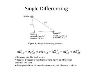
Single Differencing. • Removes satellite clock errors • Reduces troposphere and ionosphere delays to differential between two sites • Gives you relative distance between sites, not absolute position. Double Differencing. • Receiver clock error is gone

Single Differencing
E N D
Presentation Transcript
Single Differencing • Removes satellite clock errors • Reduces troposphere and ionosphere delays to differential between two sites • Gives you relative distance between sites, not absolute position
Double Differencing • Receiver clock error is gone • Random errors are increased (e.g., multipath, measurement noise) • Double difference phase ambiguity is an integer
Ambiguity Resolution: why Average east repeatability – bias free = 3.3 mm - bias-fixed = 2.7 mm 78 stations distributed around the globe
Ambiguity resolution • Resolving integer ambiguity converts carrier phase biases into ultraprecisepsuedorange Blewitt, G., “Carrier Phase Ambiguity Resolution for the Global Positioning System Applied to Geodetic Baselines up to 2000 km”, J. Geophysical Research, 1989
Double Differencing • Satellite and clock errors are gone • Random errors are increased (e.g., multipath, measurement noise) • Double difference phase ambiguity is a true integer: removes uncalibrated components of phase delay for receiver and satellite
Ambiguity Resolution How do we go about solving for N? What we end up doing is solving for “widelane” and “narrowlane” biases. • First, form “widelane” linear combination of phase observables:
Ambiguity resolution • Use pseudorange to calibrate widelane, solve for b • Computed at each data point, time averaged real value is taken • Form double differenced widelane • Independent of knowledge of orbits, station locations • Dependent on common visibility of satellites.
Ambiguity resolution • Then solve for narrowlane ambiguities • Narrowlane is ionospheric free combination:
Analysis Software • What are some differences between GIPSY and GAMIT?
High precision GPS for Geodesy • Use precise orbit products (e.g., IGS or JPL) • Use specialized modeling software • GAMIT/GLOBK • GIPSY-OASIS • BERNESE • These software packages will • Estimate integer ambiguities • Reduces rms of East component significantly • Model physical processes that effect precise positioning, such as those discussed so far plus • Solid Earth Tides • Polar Motion, Length of Day • Ocean loading • Relativistic effects • Antenna phase center variations
High precision GPS for Geodesy • Produce daily station positions with 2-3 mm horizontal repeatability, 10 mm vertical. • Can improve these stats by removing common mode error.
How to get started? • Don’t need to process data yourself? • APPS (replaces auto-gipsy) http://apps.gdgps.net/ • PBO Analysis centers • Acquire software • GIPSY: https://gipsy-oasis.jpl.nasa.gov/ • GAMIT: http://www-gpsg.mit.edu/~simon/gtgk/ • Learn software basics: • UNAVCO short course on GAMIT : • http://www.unavco.org/edu_outreach/shortcourses.html • No regular courses offered on GIPSY currently • read documentation & work with JPL’ers
Processing Overview • Get Daily dual frequency GPS observations from a network of stations (or could be 1 station) - “RINEX files” • Edit the data for outliers, losses of lock by the receiver (cycle slips) • Model the observations • Fixing orbits and clocks of the satellites, polar motions, etc. • Modeling tidal effects, propagation delays, etc. • Estimate station coordinates and other station parameters • Solutions • Station coordinates and covariances • Tropospheres as a functions of time • Phase biases as functions of satellite-station pairs and time • Station Clocks • Residuals between model and phase, pseudorange • Repeat for next day of data
A bit on RINEX files • GPS data are stored in a binary format on the receiver. • Data are downloaded and converted into ascii format, RINEX. • Type of observations: • L1 and L2 are the carrier phase data in cycles. • D1 and D2 are doppler frequencies. • C1 is the C/A code pseudorange on L1 (meters) • P1 and P2 are L1/L2 pseudoranges using the Pcode (meters) • S1 and S2 are signal to noise ratios (not always available)
Processing Steps • Collect Data (campaign or continuous) • Raw data is converted from binary to RINEX format • Keep track of metadata • Equipment used • Antenna heights • Get any additional data and metadata from archive • ftp and web services • Get precise orbits, clocks, and EOP from an archive/provider • E.g, ftp://sideshow.jpl.nasa.gov/pub/gipsy/products • Decide on • Solution rate • Data rates are usually 30 sec • Solution rates are usually daily • Network vs. Point Positioning • More CPU, memory • Faster, independent • Do I need those biases fixed? • How big is the signal? • What is the solution rate? • How long is the time series?
Processing Steps • Process GPS observables • Fixed orbits and clocks? • Estimating • Station positions • Nuisance parameters (i. e. clocks, trops, etc.) • Assess quality of estimates • Are the formal errors reasonable? • Are the values of the parameters reasonable? • Are the residuals nominal? • Were there a lot of data outliers and/or phase breaks ? • Post-Process • Time series of station positions for • Scientific signals • Geodetic studies
GIPSY: How its used /goa/bin/gd2p.pl -i chwk0010.00o -w_elmin 15 -d 2000-01-01 \ -n chwk -stop_before wash \ -tdp_in /sggs0/tdpfilein2 \ -orb_clk "flinn /tmp/orbits/“ \ -add_ocnld -no_del_shad
Analysis of Very Large GPS Data Sets • Challenge to analyze the large amount of data efficiently: • - 10 years of data from 1000+ station network. • - Almost 2 years to process data set using single CPU. • Solved problem by developing Network Processor: • - Produces bias-fixed solutions using GIPSY on cluster computers. • - Using 250 dual processor nodes, can re-analyze entire GEONET data set in under 2 days.
Reference Frame • The Terrestrial RF provides the stable coordinate system that allows us to link measurements over space and time. • Cartesian Coordinate System • Earth Centered Earth Fixed • Defined by station coordinates and station velocities • Velocities usually linear with time • Not really true for any point on the Earth • Some examples: • International Terrestrial Reference Frame (ITRF) • http://itrf.ensg.ign.fr/ITRF_solutions/2005/ITRF2005.php • Stable North American Reference Frame (SNARF) • http://www.unavco.org/research_science/workinggroups_projects/snarf/snarf.html
ITRF • International Terrestrial Reference Frame • Space geodesy based • Satellite Laser Ranging for geocenter • Very Long Baseline Interferometery (VLBI) for scale • VLBI for celestial orientation • GPS and DORIS (and VLBI and SLR) for coordinate positions and velocities • DORIS is a French system for positioning of TOPEX/Poseidon & Jason satellites • Identical to WGS84 at the meter level
Why does ITRF use multiple techniques? • High precision geodesy is very challenging • Accuracy of 1 part per billion • Fundamentally different observations with unique capabilities • Together provide cross validation and increased accuracy
Reference Frame: ITRF05 • Defined by station coordinates and velocities • Coordinates at reference epoch: Jan 1, 2005.
Reference Frame: ITRF05 • Defined by station coordinates and velocities • Coordinates at reference epoch: Jan 1, 2005.
Reference Frame: SNARF • Example of “local” reference frame definition • Plate boundary velocities in ITRF05 aren’t as easy to interpret:
Reference Frame: SNARF • Need sites on stable NA. Some challenges: • Glacial Isostatic Adjustment is significant signal in stable interior • Historically, not as many sites in stable regions • Shorter time series for defining velocities • Sites are installed for navigation/surveying instead of tectonic purposes • Similar to ITRF, combine time series from different analysis centers • Different from ITRF, only uses GPS time series
SNARF and GIA • Dominant vertical signal • Need to model in order to determine translation between SNARF and ITRF
SNARF: Accounting for GIA • Horizontal effects not very well constrained M. Tamisea
Plate Boundary Observatory Velocities From GPS Explorer website: http://geoapp03.ucsd.edu/gridsphere/gridsphere
Combining different GPS velocities • Velocity fields are in different realizations of frame • Need to make sure solutions are loosely constrained • Difficult to account for from different analysis software • Need to put all solutions into a common reference frame • Helmert’s Transformation • 7-Parameters • Scale • Translation • Rotations
If you see a signal in a GPS time series, what should you ask? • Were precise techniques applied? • Is the equipment and software recognized for high precision work? • Were the orbits high precision orbits? • Is the reference frame a high precision frame? • Are there unmodeled and systematic errors? • Are there correlations between the height and vertical estimates? • Are the residuals, chi-square, and other metrics of fit reasonable? • Could this be some non-tectonic phenomena? • A strange tropospheric effect? • A vertical and/or horizontal signal? • Changes at the GPS site • Is the signal regional or only seen on one station?
Other things to care about • Was a quality source of orbits and clocks used? • Was a fancy estimation strategy used? • Was the solution regionally filtered? • Are there regionally correlated signals? • Tectonic source? • Orbit error? • Are the results consistent with expectations from best practices? • Positions • 3, 5, 6 mm (Bias free) • 1, 1, 4 mm (Bias fixed) • Velocities • 0.2 – 0.3 mm/yr over several years