Download
1 / 32
320 likes | 449 Views
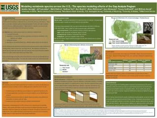
Modeling species distribution using species-environment relationships. Fabio Corsi. Istituto di Ecologia Applicata Via L.Spallanzani, 32 00161 Rome ITALY email: iea @mclink.it. Conservation Needs. Broad scale planning (eventually global) Metapopulation approach

E N D
Modeling species distribution using species-environment relationships Fabio Corsi Istituto di Ecologia Applicata Via L.Spallanzani, 32 00161 Rome ITALY email: iea@mclink.it
Conservation Needs • Broad scale planning (eventually global) • Metapopulation approach • Identification of core areas and corridors • …. Which imply • Detailed knowledge on actual species distribution • Extensive data on species ecology and biology • Spatially explicit predicting tools
The information “space” • data are: • fragmented • localised • on average, of modest quality Can we use them for broad scale planning?
The answer is a set of new questions • Can we extrapolate existing knowledge to the entire continent? • Under which assumptions? • For which use?
Can we extrapolate existing knowledge to the entire continent? • Yes, using modeling techniques which • enable to extrapolate from limited data new information • are cost effective • produce updateable distributions • define a repeatable approach
Spatial Modeling Geographic space Geographic space Environmental space En En E2 E2 E1 E1 E1 En E2 Feedback
Under which assumptions? • Species distribution is influenced by available environmental data (e.g. test for randomness of point data; Mantel test) • Local variations of these relationships throughout the study area can be neglected (e.g. stratification) • Available data are sufficient to define species-environment relationships (field validation, sensitivity analysis, hope and fate )
Alternatives Interpolation Quantitative data Distribution Semivariogram structure Feedback
For which use? • Application of results include, but are not limited to: • Identify potential/critical corridors • Predict areas of major conflicts • Assessment of conservation scenarios and management options on a cost/benefit basis (zoning system) • Include spatial elements in a PHVA • …..
“Blotch” distribution • The polygon defining the distribution range of the species as interpreted by the specialist based on her/his knowledge • The environmental requirements of the species are synthesized directly into the drawing itself
Selection Avoidance Deterministic overlay • The analysis of the environmental space is synthesized by the expert knowledge (deductive approach based on known ecological preferences) • Simple overlay of environmental variables layers • The goal is to describe the distribution within the “blotch” perimeter, showing the areas of expected occurrence. • Mostly categorical models of suitability
Observations a ... b c ... 1 60 12 .5 ... 31 20 2 .7 ... 3 .2 7 50 ... ... ... ... ... F2 F1 Habitat Suitability Statistical overlay • Formal analysis of the environmental space defined by the available variables • Result of previous analysis control the overlay process. • The goal is to describe the variation of suitability within the “blotch” • Continuous suitability rank surface
Examples • Models developed at regional scale for the large Italian carnivores and major ungulate species Available data • Extent of Occurrence of each species • known territories and point locations from previous studies (e.g. radio tracking, direct investigations etc.) • land cover maps, digital terrain model, population densities, ungulates distributions, protected areas, sheep and goats densities
The method (step 1) • Environmental data pre-processed with map algebra to account for individuals awareness of the environment
x x = f(x in blue cells) The method (step 1) • Surface of the circular window is equal to the average size of the territories and/or home range • To each cell of the study area is assigned a value which is a function of the surrounding cells
Building the model (Step 2) • Environmental characterisation of known species locations based on available environmental variables L1 L1 L2 L3 ...Ln L3 Ln Locations E11 E12 E13 E1n L2 E21 E22 E23 E2n En1 En2 En3 Enn { E1 E2 En Environmental variables
E2 E1 En Building the model (Step 2) • Calculating the species “ecological signature” E1 S E1 / n = E1 S E2 / n = E2 ... S En / n = En L1 L2 L3 … Ln E11 E12 E13 E1n E21 E22 E23 E2n En1 En2 En3 Enn En E2
Building the model (Step 3) • Calculating the distance of each portion of the study area from the ecological signature in the environmental variables space E1 Px Px E1x E2x ... Enx Ecological Distance E1x E2x Enx En E2
VE1 CE1E2 CE1En CE2E1 VE2 CE2En CEnE1 CEnE2 VEn The method (Step 3) • Species “ecological signature” calculated as the vector of means and the variance-covariance matrix S Variance-covariance matrix m Vector of means L1 L2 L3…. Ln E11 E12 E13 E1n E1 E2 ... En E21 E22 E23 E2n & En1 En2 En3 Enn
The method (Step 3) • Using the above definition of “ecological signature”, distances can be calculated using the Mahalanobis Distance D = Mahalanobis distance (environmental distance) at point x x = vector of environmental variables measured in x m = vector of the means S = variance-covariance matrix
Mahalanobis distance • takes into account not only the average value but also its variance and the covariance of the variables measured • accounts for ranges of acceptability (variance) of the measured variables • compensates for interactions (covariance) between variables • dimensionless • if the variables are normally distributed, can be readily converted to probabilities using the 2 density function
Map production • The mean (m) and standard deviation (s) of the Ecological Distance is calculated for the territories and locations • The Ecological Distance surface is partitioned according to the following threshold: • m, m + 1s ,m + 2s, m + 4s, m + 8s, m + 16s • First three classes account for more than 95% of variability (assuming a normal distribution)
The Extent of Occurrence • Accounts for variables that influence the species distribution but cannot easily be included in the analysis, such as: • historical constraints • behavioural patters • … • Mapped results are interpreted as expected within the EO and potential outside the EO
Results • Environmental suitability model for the Wolf
Results • Cumulative frequency distributions log-normal distribution of dead wolves environmental distance classes in the study area
Results • Environmental suitability model for the Lynx
Results • Environmental suitability model for the Lynx (boarder between France, Switzerland and Italy)
Results • Environmental suitability model for the Bear
Results • Environmental suitability model for the Deer
Towards a model for biodiversity • Biodiversity distribution models may derive from: • deterministic overlay of suitability models • the analysis of the environmental suitability space Species 1 Classification Clustering Species n … Species 2
Classification • Map showing the result of the principal component analysis on the suitability maps of the 3 species of large carnivores in the Alps
Alternatives Interpolation Quantitative data Distribution Semivariogram structure Feedback