Time Series Data
430 likes | 767 Views
Time Series Data. y t = b 0 + b 1 x t1 + . . .+ b k x tk + u t Basic Analysis. Time Series vs. Cross Sectional. Time series data has a temporal ordering, unlike cross-section data

Time Series Data
E N D
Presentation Transcript
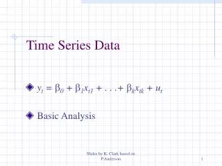
Time Series Data yt = b0 + b1xt1 + . . .+ bkxtk + ut Basic Analysis Slides by K. Clark based on P.Anderson
Time Series vs. Cross Sectional • Time series data has a temporal ordering, unlike cross-section data • Will need to alter some of our assumptions to take into account that we no longer have a random sample of individuals • Instead, we have one realization of a stochastic (i.e. random) process
Examples of Time Series Models • A static model relates contemporaneous variables: yt = b0 + b1zt + ut • A finite distributed lag (FDL) model allows one or more variables to affect y with a lag: • yt = a0 + d0zt + d1zt-1 + d2zt-2 + ut • More generally, a finite distributed lag model of order q will include q lags of z
Lagged Dependent Variable Models • Another common type of time series model is where one or more lags of the dependent variable appear, e.g. • yt = a0 + d0yt-1 + d1yt-2 + d2yt-3 + ut • Such models are not considered in ES5611 but reappear in ES5622 • Here they are ruled out by assumption TS.2
Assumptions for Unbiasedness • [TS.1] Assume a model that is linear in parameters: yt = b0 + b1xt1 + . . .+ bkxtk + ut • [TS.2] Zero conditional mean assumption: E(ut|X) = 0, t = 1, 2, …, n • Note that this implies the error term in any given period is uncorrelated with the explanatory variables in all time periods • This assumption also called strict exogeneity
Assumptions (continued) • An alternative assumption, more parallel to the cross-sectional case, is E(ut|xt) = 0 • This assumption would imply the x’s are contemporaneously exogenous • Contemporaneous exogeneity will only be sufficient in large samples
Assumptions (continued) • [TS.3] Assume that no x is constant, and that there is no perfect collinearity • Note we have skipped the assumption of a random sample • The key impact of the random sample assumption is that each ui is independent • Our strict exogeneity assumption takes care of it in this case
Unbiasedness of OLS • Based on these 3 assumptions, when using time-series data, the OLS estimators are unbiased • Omitted variable bias can be analyzed in the same manner as in the cross-section case
Variances of OLS Estimators • Just as in the cross-section case, we need to add an assumption of homoskedasticity in order to be able to derive variances • [TS.4] Assume Var(ut|X) = Var(ut) = s2 • Thus, the error variance is independent of all the x’s, and it is constant over time • [TS.5] Assume no serial correlation: Cov(ut,us| X) = 0 for t s
OLS Variances (continued) • Under these 5 assumptions, the OLS variances in the time-series case are the same as in the cross-section case. Also, • The estimator of s2 is the same • OLS remains BLUE (Gauss-Markov) • With the additional assumption of normal errors, inference is the same
Example using Microfit (10.3) • Microfit 4 available on all networked computers • Econometric package geared towards time series analysis • Mainly menu driven package • Has some quirks • Practice exercise and handout on Web page but not expecting you to become proficient - more in ES5622
Example using Microfit (cont’d) • Castillo-Freeman and Freeman (1992): effect of minimum wage on employment in Puerto Rico • Variables: prepop - employment rate, mincov - ‘importance’ of minimum wage, • Simple Model: • log(prepop) = b0 + b1log(mincov) + u • Clear prediction from economic theory of sign of b1
Microfit output - page 1 Ordinary Least Squares Estimation ******************************************************************************* Dependent variable is LPREPOP 38 observations used for estimation from 1950 to 1987 ******************************************************************************* Regressor Coefficient Standard Error T-Ratio[Prob] CONSTANT -1.1598 .027281 -42.5120[.000] LMINCOV -.16296 .019481 -8.3650[.000] ******************************************************************************* R-Squared .66029 R-Bar-Squared .65085 S.E. of Regression .054939 F-stat. F( 1, 36) 69.9728[.000] Mean of Dependent Variable -.94407 S.D. of Dependent Variable .092978 Residual Sum of Squares .10866 Equation Log-likelihood 57.3657 Akaike Info. Criterion 55.3657 Schwarz Bayesian Criterion 53.7282 DW-statistic .34147 ******************************************************************************* • Note where all the usual stuff is
Microfit output - page 2 Diagnostic Tests ******************************************************************************* * Test Statistics * LM Version * F Version * ******************************************************************************* * * * * * A:Serial Correlation*CHSQ( 1)= 25.8741[.000]*F( 1, 35)= 74.6828[.000]* * * * * * B:Functional Form *CHSQ( 1)= 2.8662[.090]*F( 1, 35)= 2.8553[.100]* * * * * * C:Normality *CHSQ( 2)= .071873[.965]* Not applicable * * * * * * D:Heteroscedasticity*CHSQ( 1)= 4.3213[.038]*F( 1, 36)= 4.6192[.038]* ******************************************************************************* A:Lagrange multiplier test of residual serial correlation B:Ramsey's RESET test using the square of the fitted values C:Based on a test of skewness and kurtosis of residuals D:Based on the regression of squared residuals on squared fitted values
Trending Time Series • Economic time series often have a trend • Just because 2 series are trending together, we can’t assume that the relation is causal • Often, both will be trending because of other unobserved factors - leads to spurious regression • Even if those factors are unobserved, we can control for them by directly controlling for the trend
Example - trending data • UK aggregate consumption and income 1948-85, annual data • Note extremely high correlation in scatter plot • R2 = 0.9974
Trends (continued) • One possibility is a linear trend, which can be modeled as yt = a0 + a1t + et, t = 1, 2, … • Another possibility is an exponential trend, which can be modeled as log(yt) = a0 + a1t + et, t = 1, 2, … • Another possibility is a quadratic trend, which can be modeled as yt = a0 + a1t + a2t2 + et, t = 1, 2, …
Detrending • Adding a linear trend term to a regression is the same thing as using “detrended” series in a regression • Detrending a series involves regressing each variable in the model on t • The residuals form the detrended series • Basically, the trend has been partialled out
Detrending (continued) • An advantage to actually detrending the data (vs. adding a trend) involves the calculation of goodness of fit • Time-series regressions tend to have very high R2, as the trend is well explained • The R2 from a regression on detrended data better reflects how well the xt’s explain yt
Example again • Define time trend variable, t • Original model: Model with trend:
Example (cont’d) • Scatter plot of detrended series • R2 = 0.7868 • Still high but a more accurate measure of how well Y explains C • However, these data may be highly persistent and simple methods not appropriate (Wooldridge, Ch.11, ES5622)
Time Series Data yt = b0 + b1xt1 + . . .+ bkxtk + ut Serial Correlation Slides by K. Clark based on P.Anderson
Serial Correlation defined • Serial correlation (autocorrelation) is where TS.5 does not hold • Cov(ut,us¦X) 0 for t s. • A particular form of serial correlation is extremely common in time series data • This is because ‘shocks’ tend to persist through time
Implications of Serial Correlation • Unbiasedness (or consistency) of OLS does not depend on TS.5 • However OLS is no longer BLUE when serial correlation is present • And OLS variances and standard errors are biased • Hence usual inference procedures are not valid
The AR(1) Process • First order autoregressive error process a useful model of serial correlation • yt = b0 + b1xt1 + . . .+ bkxtk + ut • ut = rut-1 + et |ρ| < 1 • where et are uncorrelated random variables with mean 0 and variance σe2 • Typically expect r > 0in economic data • Positive serial correlation
The AR(1) Process • E(ut) = 0 • Var(ut) = σe2/(1-r2) • Cov(ut, ut+j) = rjVar(ut) • Corr(ut, ut+j) = rj • So the error term is zero mean, homoscedastic but has serial correlation which is positive if ρ > 0
Estimator variance: simple regression This is not equal to the usual formula since Cov(ut, us) 0 in the presence of serial correlation
Testing for AR(1) Serial Correlation • Want to be able to test for whether the errors are serially correlated or not • Want to test H0: r = 0 in ut = rut-1 + et, t =2,…, n, where ut is the regression model error term • With strictly exogenous regressors, an asymptotically valid test is very straightforward – simply regress the residuals on lagged residuals and use a t-test
Testing for AR(1) Serial Correlation (continued) • An alternative is the Durbin-Watson (DW) statistic, which is calculated by many packages • If the DW statistic is around 2, then we can reject serial correlation, while if it is significantly < 2 we cannot reject • Critical values are in the form of ‘bounds’: reject if DW<dL, do not reject if DW>dU, inconclusive otherwise. Tables available.
Testing for AR(1) Serial Correlation (continued) • Note that the t-test is only valid asymptotically while DW has an exact distribution under classical assumptions including normality. • If the regressors are not strictly exogenous, then neither the t nor DW test are valid • Instead regress the residuals (or y) on the lagged residuals and all of the x’s and use a t-test
Testing for Higher Order S.C. • Can test for AR(q) serial correlation in the same basic manner as AR(1) • Just include q lags of the residuals in the regression and test for joint significance • Can use F test or LM test, where the LM version is called a Breusch-Godfrey test and is (n-q)R2 using R2 from auxiliary (residual) regression
Example • In the Puerto Rico minimum wage example, DW = 0.3415 • dL = 1.535 so we can reject H0: r = 0 against H1: r > 0 • Assuming strict exogeneity, an auxiliary regression gives: • Hence reject H0 • S/C is present
Correcting for Serial Correlation • Start with case of strictly exogenous regressors, and maintain all G-M assumptions except no serial correlation • Assume errors follow AR(1) so • ut = rut-1 + et, t =2,…, n • Var(ut) = s2e/(1-r2) • We need to try and transform the equation so we have no serial correlation in the errors
Correcting for S.C. (continued) • Use a simple regression model for convenience: • Consider that since yt = b0 + b1xt + ut , then • yt-1 = b0 + b1xt-1 + ut-1 • If you multiply the second equation by r, and subtract if from the first you get • yt– r yt-1 = (1– r)b0 + b1(xt – r xt-1) + et , since et= ut– r ut-1 • This quasi-differencing results in a model without serial correlation
Feasible GLS Estimation • OLS applied to the transformed model is GLS and is BLUE • Problem: don’t know r, so we need to get an estimate first • Can use estimate obtained from regressing residuals on lagged residuals without an intercept • This procedure is called Cochrane-Orcutt estimation
Feasible GLS Estimation • One slight problem with Cochrane-Orcutt is that we lose an observation (t = 1) • The Prais-Winsten method corrects this by multiplying the first observation by (1-ρ2)1/2 and including it in the model • Asymptotically the two methods are equivalent • But in small sample, time-series applications two methods can get different answers
Feasible GLS (continued) • Often both Cochrane-Orcutt and Prais-Winsten are implemented iteratively • This basic method can be extended to allow for higher order serial correlation, AR(q) • Most statistical packages including Microfit will automatically allow for the estimation of such models without having to do the quasi-differencing by hand
FGLS versus OLS • In the presence of serial correlation OLS is unbiased, consistent but inefficient • FGLS is consistent and more efficient than OLS if serial correlation is present and the regressors are strictly exogenous • However OLS is consistent under a weaker set of assumptions than FGLS • So choice of estimator depends on weighing up different criteria
Serial Correlation-Robust Standard Errors • It’s possible to calculate serial correlation-robust standard errors, along the same lines as heteroskedasticity robust standard errors • Idea is to scale the OLS standard errors to take into account serial correlation • The details of this are beyond our scope - the method is implemented in Microfit where it goes by the name of Newey-West
Example • In Puerto Rico minimum wage example: • found serial correlation • compute Cochrane-Orcutt estimates by hand • find iterated C-O estimates • Find Newey-West s/c robust standard errors • Demonstrate in Microfit • Results compared on next slide
Next Week and beyond • Next Week (8/12/03): Go through mock exam answers in usual lecture time and place • KC will keep office hours (Wed 10-12) while the University is open • Email for appointment outside these times (ken.clark@man.ac.uk) • Check with tutors for their availability
Next Semester - ES5622 • 5 lectures on Cross Section econometrics by Dr Martyn Andrews - Wooldridge, Chapter 7 is good preliminary reading • 5 lectures on Time Series methods by Dr Simon Peters, Wooldridge Chapters 10-12 good preliminary reading, other references mentioned in lectures
