Download
1 / 53
530 likes | 683 Views
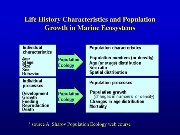
Life History Characteristics and Population Growth in Marine Ecosystems. 1 source A. Sharov Population Ecology web course. Population Ecology. A population is a group of individuals of the same species that occupy a specified region at a specified time.

E N D
Life History Characteristics and Population Growth in Marine Ecosystems 1 source A. Sharov Population Ecology web course
Population Ecology A population is a group of individuals of the same species that occupy a specified region at a specified time. Key questions of population ecology include: What is the size of a population? What is the potential for growth in the population? What form will growth take?
Population Growth • N(t+1) = N(t) + B(t) + I(t) – D(t)– E(t) where, N=number of individuals, B=births, I=immigrations, D=deaths, and E=emigrations ------BIDE
Overview of Ecological Theory • Population Growth and regulation • biological populations have great potential for increase, however, populations never realize this potential. There appears to be some factors (e.g., food limitation, war) that keep population regulation within some definable limits.
Population growth models geometric -- used when there is a discrete breeding season exponential-- used when populations are growing continuously
Population growth models geometric the ratio of the population in one year to the population in the previous year the rate of geometric growth =
Geometric Growth Model • Population growth incrementally • Geometric Growth rate () • Ratio of the population in one year to that in the preceding year • = N(1)/N(0) • = er Where r=b-d
Assumptions of the Geometric Growth Model • Population is growing under optimum conditions • Population has discrete generations (live and die at the same time) • Breeds only one time per year (semelparous-salmon) • Focuses only on females (millions of sperm/egg)
Population growth models exponential the contribution of each individual to population growth the rate of change in population size the number of individuals in population = x
Population growth models exponential dN/dt = rN N(t) = N(o)ert where, N=number r = (birth – death) t=time
r = births - deaths Components of the environment that affect birth or death rate will also affect r. Therefore, each environment a population lives in might produce a different r. And, if r can vary, it can be subject to natural selection and selective pressures can shape the values of r in different situations. Intrinsic Growth Rate
Intrinsic Rates of Increase • On average, small organisms have higher rates of per capita increase and more variable populations than large organisms.
Small marine invertebrate: • Pops. of pelagic tunicates (Thalia democratica) grow at exponential rates in response to phytoplankton blooms. • Life cycle involves a mixture of sexual and asexual reproduction • Increase pop. size dramatically due to extremely high reproductive rates. Large marine mammal: • Female gray whales (E. robustus) give birth, on average, every other year • Reilly et al. (1983) estimated 2.5% growth for California population in 1967-1980
Assumptions of the exponential growth model • Reproduction is continuous (no seasonality) • All organisms are identical (e.g., no age structure) • Environment is constant in space and time (resources are unlimited)
Logistic Growth • Because of “Environmental Resistance” population growth decreases as density reaches a “carrying capacity” or K • Graph of individuals vs. time yields a sigmoid or S-curved growth curve • Reproductive time lag causes population to overshoot K • Population will not be unvarying due to resources (prey) and predator effects
An example with barnacles (Connell 1961): K is determined largely by the amount of space available on rocks for attachment barnacle (Balanus balanoides)
Population growth models logistic dN/dt = rN(K-N/K) N(t) = K/1 + ea-rt r = birth – death K=carrying capacity a= integration constant
Environmental Resistance • Factors that reduce the ability of populations to increase in size • Abiotic Contributing Factors: • Unfavorable light • Unfavorable Temperatures • Unfavorable chemical environment - nutrients • Biotic Contributing Factors: • Low reproductive rate • Specialized niche • Inability to migrate or disperse • Inadequate defense mechanisms
Two Schools of Thought Density independent school - changes in physical environmental factors (generally climatic changes); which lead to dramatic shifts in populations. Density dependent school - work with larger organisms (vertebrates) or sessile organisms (barnacles); biotic interactions and their importance (competition, predation, or parasitism) *large controversy over the relative importance of these factors
Density-dependent responses Density independent Population or individual parameter Density dependent Density
r and K selection r vs K (intrinsic growth rate) (carrying capacity) Any organism has three categories that it needs to allocate energy to: • Growth • Reproduction • Maintenance (basal metabolic activity; building of bone and supporting structures)
r selected traits • rapid development • small body • early reproduction • semelparity • (single reproduction) • K selected traits • slow development • large body • delayed reproduction • iteroparity • (repeated reproduction) Thought to divide invertebrates from vertebrates; many exceptions; all are relative (barnacle to whales) Overgeneralization, but it does seem to have some usefulness in organizing thinking
Hypothetical metapopulation dynamics. Closed circles represent habitat patches, dots represent individual plants or animals. Arrows indicate dispersal between patches. Over time the regional metapopulation changes less than each local population.
Demography • Demography is the study of the vital statistics of a population
Demography • Life Tables are the main tool for demographers, and they have 2 main components • Survivorship schedule – average # of individuals that survive to any particular age • Fertility schedule (fecundity) – average # of daughters produced by one female on each life stage Population size = double the # of daughters born to each female (assumes the same # of sons as # of daughters)
Types of Life Tables • Static life table – calculated on a cross section of the population at a specific time. Estimate # of individuals from each age group and look at # of deaths for each age group • 2. Cohort life table – follow a cohort through out their life and record the # of individuals surviving to each stage. • Both will give the same results if birth rate and death rate remain constant
Age Determination-Otoliths 5 • Otoliths are composed primarily of aragonite, which is a form of calcium carbonate • Readers count bands 4 3 2 1
Coral growth rings • Each of the light/dark bands in this x-ray of a cross-section of a coral core formed during a year of growth
Seagrass Demography Leaves Short- Shoot Stem Leaf Scars (plastochrone intervals) Rhizome scars
Age Structure Diagrams Positive Growth Zero Growth Negative Growth (ZPG) Pyramid Shape Vertical Edges Inverted Pyramid
Survivorship table Using these data , calculate the proportion of population surviving at the start of each period ( l ) . x x #barnacles at start ( Prop. Surviving (N /N ) x O 0 12 100% (12/12) 1 6 50% (6/12) 2 3 25% (3/12) 3 1 8% (1/1 2)
Fertility Schedule Provides the average number of daughters Ø produced by one female at each particular age Customarily, only females are tracked, since it Ø is virtually impossible to measure the fecundity of males It is assumed that the male population wil l Ø grow the same way the female population grow
Net Reproductive Rate (Ro) Is the average number of offspring produced by Ø each female during her entire lifetime Can be calculated by summing the products of Ø the survivorship and fecundity schedules from birth to death When Ro<1, the population declines; when Ø Ro=1, the population is stable; and when Ro> 1, the population increases
A highly significant way of reducing fecundity is increase the age of first reproduction Population 1 Population 2 X(age) Lx mx X(age) Lx mx 0 1.0 0 0 1.0 0 1 0.5 1.0 1 0.5 0 2 0.4 3.0 2 0.4 1 3 0.2 0 3 0.2 3 R o=1.7 Ro=1.0
Surv ivorship Table ( ) and Fertility Table ( ) for Women in l b x x the United States, 1989 No. Female Offspring per Proportion Female Aged Surviving to Age Midpoint or x per 5 - Year Product of l x Up Pivotal Age x Pivotal Age l Time Unit ( b ) and b x x x 0 - 9 5.0 0.9895 0.0 0.0 10 - 14 12.5 0.9879 0.0020 0.0020 15 - 19 17.5 0.9861 0.1233 0.1216 20 - 24 22.5 0.9834 0.2638 0.2594 25 - 29 27.5 0.9802 0.2772 0.2717 30 - 34 32.5 0.9765 0.1807 0.1765 35 - 39 37.5 0.9712 0.0650 0.0631 40 - 44 42.5 0.9643 0.0125 0.0121 45 - 49 47.5 0.9528 0.0005 0.0005 and above ---- ---- 0.0 0.0 l b = 0.9069 R = x x 0
Life History Components • The important components include: • the age and size at which reproduction occurs • the relative apportionment of energy to reproduction, growth, survivorship, and predator avoidance • production of many small or a few large offspring • the age of first reproduction • age of death
Life History Strategies • Assumptions: • Natural selection will produce a life history tactic (strategy) that will maximize the individual fitness of the organism under study by optimizing the allocation of energy between these function. • Fixed amounts of energy (investing energy in one will take it from another) The goal of life history strategy: to predict the characteristics of any organism that you might expect to find under any given set of conditions
Examples of life history considerations • If environmental conditions change, what effect might this that have on growth or reproduction? • Should most energy be allocated to growth in year 1 or should more energy be put into factors that protect you from predators or to reproduction? • How many young should be produced? • How many reproductive events would best take place during an organism’s life to maximize fitness? • Should organisms allocate energy to care for young?
Stressful Environments In area where large amounts of density independent mortality occurs (catastrophic events that cause high mortality; weather or climatic) r selection dominates: organisms should survive here when they allocate a lot of energy to early reproduction, rapid growth, and dispersal to new habitats
Stable Environments When K selection dominates: populations will increase until they approach K where competition will increase. In this situation good competitors will be selectively favored (density dependent mortality) organisms should survive when they allocate energy to slow development, delayed reproduction, usually large and may have frequent reproductive events throughout life.
Bet hedging Occurs where environmental conditions vary greatly and juveniles or adults are subject to high density independent mortality If high juvenile mortality: smaller reproductive output, smaller litters at any given time, and longer lived organisms If high adult mortality: increased reproductive effect, larger litters, and shorter lifespan
Reproductive Strategies • Semelparity • Favored by stable, predictable environments • less energy required for maintenance • more energy devoted to reproduction • produces cohorts of similar-aged young
Iteroparity – offspring are produced multiple times during an organisms lifetime; found in most marine organisms • Favored by unstable, non-predictable environments • - likened to “bet-hedging” • - survival of juveniles is low and unpredictable, thus selection favors repeated reproduction and long reproductive life • - tends to produce young of different ages • - much variation in # of clutches and size of clutch
Egg Size and Number in Fish • Fish show more variation in life-history than any other group of animals. • clutch size (# of offspring per brood): • ranges from 1-2 live births produced by mako shark (Isurus oxyrinchus) • to 600,000,000 eggs produced by ocean sunfish (Mako mako)
Life History Variation Among Fish Species Gunderson (1997) studied adult survival and reproductive effort of several fish spp. • Reproductive effort measured as gonadosomatic index (GSI) = (ovary weight / body weight) x (# of batches of offspring produced per year) • Species with higher rates of mortality show higher relative reproductive effort
Modular growth • Modular growth occurs when organisms reproduce asexually by increasing the # of modules they possess (e.g., corals, bryozoans, and cnidarians). • r and K have no meaning for these organisms; colonial growth allows them to have incredibly long life spans. • A common theme is that under stressful conditions organisms with modular growth turn on sexual reproduction for dispersal.