Huffman code and ID3

1. CS 157 B Lecture 18 Huffman code and ID3 Prof. Sin-Min Lee Department of Computer Science

2. Data Compression • Data discussed so far have used FIXED length for representation • For data transfer (in particular), this method is inefficient. • For speed and storage efficiencies, data symbols should use the minimum number of bits possible for representation.

3. Data Compression Methods Used For Compression: • Encode high probability symbols with fewer bits • Shannon-Fano, Huffman, UNIX compact • Encode sequences of symbols with location of sequence in a dictionary • PKZIP, ARC, GIF, UNIX compress, V.42bis • Lossy compression • JPEG and MPEG

4. Data Compression Average code length Instead of the length of individual code symbols or words, we want to know the behavior of the complete information source

5. Data Compression Average code length Assume that symbols of a source alphabet {a1,a2,…,aM} are generated with probabilities p1,p2,…,pM P(ai) = pi (i = 1, 2, …, M) • Assume that each symbol of the source alphabet is encoded with codes of lengths l1,l2,…,lM

6. Data Compression Average code length Then the Average code length, L, of an information source is given by:

7. Data Compression Variable Length Bit Codings Rules: • Use minimum number of bits AND • No code is the prefix of another code AND 3. Enables left-to-right, unambiguous decoding

8. Data Compression Variable Length Bit Codings • No code is a prefix of another • For example, can’t have ‘A’ map to 10 and ‘B’ map to 100, because 10 is a prefix (the start of) 100.

9. Data Compression Variable Length Bit Codings • Enables left-to-right, unambiguous decoding • That is, if you see 10, you know it’s ‘A’, not the start of another character.

10. Data Compression Variable Length Bit Codings • Suppose ‘A’ appears 50 times in text, but ‘B’ appears only 10 times • ASCII coding assigns 8 bits per character, so total bits for ‘A’ and ‘B’ is 60 * 8 = 480 • If ‘A’ gets a 4-bit code and ‘B’ gets a 12-bit code, total is 50 * 4 + 10 * 12 = 320

11. Data Compression Variable Length Bit Codings Example: Average code length = 1.75

12. Data Compression Variable Length Bit Codings Question: Is this the best that we can get?

13. Data Compression Huffman code • Constructed by using a code tree, but starting at the leaves • A compact code constructed using the binary Huffman code construction method

14. Data Compression Huffman code Algorithm • Make a leaf node for each code symbol • Add the generation probability of each symbol to the leaf node • Take the two leaf nodes with the smallest probability and connect them into a new node • Add 1 or 0 to each of the two branches • The probability of the new node is the sum of the probabilities of the two connecting nodes • If there is only one node left, the code construction is completed. If not, go back to (2)

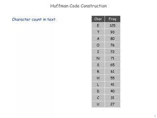
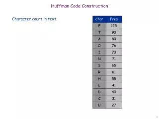
15. Data Compression Huffman code Example Character (or symbol) frequencies • A : 20% (.20) e.g., ‘A’ occurs 20 times in a 100 character document, 1000 times in a 5000 character document, etc. • B : 9% (.09) • C : 15% (.15) • D : 11% (.11) • E : 40% (.40) • F : 5% (.05) • Also works if you use character counts • Must know frequency of every character in the document

16. Data Compression Huffman code Example • Symbols and their associated frequencies. • Now we combine the two least common symbols (those with the smallest frequencies) to make a new symbol string and corresponding frequency. E .40 B .09 F .05 D .11 A .20 C .15

17. Data Compression Huffman code Example • Here’s the result of combining symbols once. • Now repeat until you’ve combined all the symbols into a single string. E .40 BF .14 D .11 A .20 C .15 B .09 F .05

18. ABCDEF1.0 ABCDF .60 AC .35 Data Compression Huffman code Example E .40 BFD .25 BF .14 D .11 A .20 C .15 B .09 F .05

19. 0 1 0 1 1 0 0 1 0 1 Data Compression ABCDEF1.0 ABCDF .60 E .40 • Now assign 0s/1s to each branch • Codes (reading from top to bottom) • A: 010 • B: 0000 • C: 011 • D: 001 • E: 1 • F: 0001 • Note • None are prefixes of another BFD .25 AC .35 BF .14 D .11 A .20 C .15 B .09 F .05 Average Code Length = ?

20. Data Compression Huffman code • There is no unique Huffman code • Assigning 0 and 1 to the branches is arbitrary • If there are more nodes with the same probability, it doesn’t matter how they are connected • Every Huffman code has the same average code length!

21. Data Compression Huffman code Quiz: • Symbols A, B, C, D, E, F are being produced by the information source with probabilities 0.3, 0.4, 0.06, 0.1, 0.1, 0.04 respectively. What is the binary Huffman code? • A = 00, B = 1, C = 0110, D = 0100, E = 0101, F = 0111 • A = 00, B = 1, C = 01000, D = 011, E = 0101, F = 01001 • A = 11, B = 0, C = 10111, D = 100, E = 1010, F = 10110

22. Data Compression Huffman code Applied extensively: • Network data transfer • MP3 audio format • Gif image format • HDTV • Modelling algorithms

24. A decision tree is a tree in which each branch node represents a choice between a number of alternatives, and each leaf node represents a classification or decision.

28. One measure is the amount of information provided by the attribute. • Example: Suppose you are going to bet $1 on the flip of a coin. With a normal coin. You might be willing to pay up to $1 for advance knowledge of the coin flip. However, if the coin was rigged so that 99% of the time heads come up, you would bet heads with an expected value of $0.98. So, in the case of the rigged coin, you would be willing to pay less that $0.02 for advance information of the result. • The less you know the more valuable the information is. • Information theory uses this intuition.

32. We measure the entropy of a dataset,S, with respect to one attribute, in this case the target attribute, with the following calculation: where Pi is the proportion of instances in the dataset that take the ith value of the target attribute This probability measures give us an indication of how uncertain we are about the data. And we use a log2 measure as this represents how many bits we would need to use in order to specify what the class (value of the target attribute) is of a random instance.

33. Entropy Calculations If we have a set with k different values in it, we can calculate the entropy as follows: Where P(valuei) is the probability of getting the ith value when randomly selecting one from the set. So, for the set R = {a,a,a,b,b,b,b,b}

34. Using the example of the marketing data, we know that there are two classes in the data and so we use the fractions that each class represents in an entropy calculation: Entropy (S = [9/14 responses, 5/14 no responses])= -9/14 log2 9/14 - 5/14 log2 5/14 = 0.947 bits

35. Example • Initial decision tree is one node with all examples. • There are 4 +ve examples and 3 -ve examples • i.e. probability of +ve is 4/7 = 0.57; probability of -ve is 3/7 = 0.43 • Entropy is: - (0.57 * log 0.57) - (0.43 * log 0.43) = 0.99

36. Evaluate possible ways of splitting. • Try split on size which has three values: large, medium and small. • There are four instances with size = large. • There are two large positives examples and two large negative examples. • The probability of +ve is 0.5 • The entropy is: - (0.5 * log 0.5) - (0.5 * log 0.5) = 1

37. There is one small +ve and one small -ve • Entropy is: - (0.5 * log 0.5) - (0.5 * log 0.5) = 1 • There is only one medium +ve and no medium -ves, so entropy is 0. • Expected information for a split on size is: • The expected information gain is: 0.99 - 0.86 = 0.13

38. Now try splitting on colour and shape. • Colour has an information gain of 0.52 • Shape has an information gain of 0.7 • Therefore split on shape. • Repeat for all subtree

48. How do we construct the decision tree? • Basic algorithm (a greedy algorithm) • Tree is constructed in a top-down recursive divide-and-conquer manner • At start, all the training examples are at the root • Attributes are categorical (if continuous-valued, they can be discretized in advance) • Examples are partitioned recursively based on selected attributes. • Test attributes are selected on the basis of a heuristic or statistical measure (e.g., information gain) Information gain: (information before split) – (information after split)

49. Conditions for stopping partitioning • All samples for a given node belong to the same class • There are no remaining attributes for further partitioning – majority voting is employed for classifying the leaf • There are no samples left