Download

1 / 83
830 likes | 862 Views
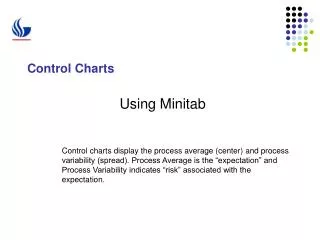
This chapter outlines the construction of variable control charts, including statistical tests and economic design. It explains how to take periodic samples from a process, plot the sample points on a control chart, and determine if the process is within limits. It also covers the different types of data, such as variable and attribute data.

E N D
CHAPTER 5: VARIABLE CONTROL CHARTS Outline • Construction of variable control charts • Some statistical tests • Economic design
Control Charts • Take periodic samples from a process • Plot the sample points on a control chart • Determine if the process is within limits • Correct the process before defects occur
Types of Data • Variable data • Product characteristic that can be measured • Length, size, weight, height, time, velocity • Attribute data • Product characteristic evaluated with a discrete choice • Good/bad, yes/no
Upper control limit Process average Lower control limit 10 9 1 2 3 4 5 6 7 8 Process Control Chart Sample number
Variation • Several types of variation are tracked with statistical methods. These include: 1. Within piece variation 2. Piece-to-piece variation (at the same time) 3. Time-to-time variation
Common Causes Chance, or common, causes are small random changes in the process that cannot be avoided. When this type of variation is suspected, production process continues as usual.
Assignable Causes Assignable causes are large variations. When this type of variation is suspected, production process is stopped and a reason for variation is sought. Average Grams (a) Mean
Assignable Causes Assignable causes are large variations. When this type of variation is suspected, production process is stopped and a reason for variation is sought. Average Grams (b) Spread
Assignable Causes Assignable causes are large variations. When this type of variation is suspected, production process is stopped and a reason for variation is sought. Average Grams (c) Shape
Mean -3 -2 -1 +1 +2 +3 68.26% 95.44% 99.74% The Normal Distribution = Standard deviation
Control Charts Assignable causes likely UCL Nominal LCL 1 2 3 Samples
Control Chart Examples UCL Nominal Variations LCL Sample number
Control Limits and Errors Type I error: Probability of searching for a cause when none exists UCL Process average LCL (a) Three-sigma limits
Control Limits and Errors Type I error: Probability of searching for a cause when none exists UCL Process average LCL (b) Two-sigma limits
Control Limits and Errors Type II error: Probability of concluding that nothing has changed UCL Shift in process average Process average LCL (a) Three-sigma limits
Control Limits and Errors Type II error: Probability of concluding that nothing has changed UCL Shift in process average Process average LCL (b) Two-sigma limits
Control Charts For Variables • Mean chart ( Chart) • Measures central tendency of a sample • Range chart (R-Chart) • Measures amount of dispersion in a sample • Each chart measures the process differently. Both the process average and process variability must be in control for the process to be in control.
Constructing a Control Chart for Variables 1. Define the problem 2. Select the quality characteristics to be measured 3. Choose a rational subgroup size to be sampled 4. Collect the data 5. Determine the trial centerline for the chart 6. Determine the trial control limits for the chart 7. Determine the trial control limits for the R chart 8. Examine the process: control chart interpretation 9. Revise the charts 10. Achieve the purpose
Example: Control Charts for Variables Slip Ring Diameter (cm) Sample 1 2 3 4 5 X R 1 5.02 5.01 4.94 4.99 4.96 4.98 0.08 2 5.01 5.03 5.07 4.95 4.96 5.00 0.12 3 4.99 5.00 4.93 4.92 4.99 4.97 0.08 4 5.03 4.91 5.01 4.98 4.89 4.96 0.14 5 4.95 4.92 5.03 5.05 5.01 4.99 0.13 6 4.97 5.06 5.06 4.96 5.03 5.01 0.10 7 5.05 5.01 5.10 4.96 4.99 5.02 0.14 8 5.09 5.10 5.00 4.99 5.08 5.05 0.11 9 5.14 5.10 4.99 5.08 5.09 5.08 0.15 10 5.01 4.98 5.08 5.07 4.99 5.03 0.10 50.09 1.15
Normal Distribution Review • If the diameters are normally distributed with a mean of 5.01 cm and a standard deviation of 0.05 cm, find the probability that the sample means are smaller than 4.98 cm or bigger than 5.02 cm.
Normal Distribution Review • If the diameters are normally distributed with a mean of 5.01 cm and a standard deviation of 0.05 cm, find the 97% confidence interval estimator of the mean (a lower value and an upper value of the sample means such that 97% sample means are between the lower and upper values).
Normal Distribution Review • Define the 3-sigma limits for sample means as follows: • What is the probability that the sample means will lie outside 3-sigma limits?
Normal Distribution Review • Note that the 3-sigma limits for sample means are different from natural tolerances which are at
Determine the Trial Control Limits for the Chart Note: The control limits are only preliminary with 10 samples. It is desirable to have at least 25 samples.
3-Sigma Control Chart Factors Sample size X-chart R-chart nA2D3D4 2 1.88 0 3.27 3 1.02 0 2.57 4 0.73 0 2.28 5 0.58 0 2.11 6 0.48 0 2.00 7 0.42 0.08 1.92 8 0.37 0.14 1.86
Examine the Process Control-Chart Interpretation • Decide if the variation is random (chance causes) or unusual (assignable causes). • A process is considered to be in a state of control, or under control, when the performance of the process falls within the statistically calculated control limits and exhibits only chance, or common, causes.
Examine the Process Control-Chart Interpretation • A control chart exhibits a state of control when: 1. Two-thirds of the points are near the center value. 2. A few of the points are close to the center value. 3. The points float back and forth across the centerline. 4. The points are balanced on both sides of the centerline. 5. There no points beyond the centerline. 6. There are no patterns or trends on the chart. • Upward/downward, oscillating trend • Change, jump, or shift in level • Runs • Recurring cycles
Revise the Charts A. Interpret the original charts B. Isolate the cause C. Take corrective action D. Revise the chart: remove any points from the calculations that have been corrected. Revise the control charts with the remaining points
Revise the Charts Where = discarded subgroup averages = number of discarded subgroups = discarded subgroup ranges
Revise the Charts The formula for the revised limits are: where, A, D1, and D2 are obtained from Appendix 2.
Reading and Exercises • Chapter 5: • Reading pp. 192-236, Problems 11-13 (2nd ed.) • Reading pp. 198-240, Problems 11-13 (3rd ed.)
CHAPTER 5: CHI-SQUARE TEST • Control chart is constructed using periodic samples from a process • It is assumed that the subgroup means are normally distributed • Chi-Square test can be used to verify if the above assumption
Chi-Square Test • The Chi-Square statistic is calculated as follows: • Where, = number of classes or intervals = observed frequency for each class or interval = expected frequency for each class or interval = sum over all classes or intervals
Chi-Square Test • If then the observed and theoretical distributions match exactly. • The larger the value of the greater the discrepancy between the observed and expected frequencies. • The statistic is computed and compared with the tabulated, critical values recorded in a table. The critical values of are tabulated by degrees of freedom, vs. the level of significance,
Chi-Square Test • The null hypothesis, H0 is that there is no significant difference between the observed and the specified theoretical distribution. • If the computed test statistic is greater than the tabulated critical value, then the H0 is rejected and it is concluded that there is enough statistical evidence to infer that the observed distribution is significantly different from the specified theoretical distribution.
Chi-Square Test • If the computed test statistic is not greater than the tabulated critical value, then the H0 is not rejected and it is concluded that there is notenough statistical evidence to infer that the observed distribution is significantly different from the specified theoretical distribution.
Chi-Square Test • The degrees of freedom, is obtained as follows • Where, = number of classes or intervals = the number of population parameters estimated from the sample. For example, if both the mean and standard of population date are unknown and are estimated using the sample date, then p = 2 • A note: When using the Chi-Square test, there must be a frequency or count of at least 5 in each class.
Example: Chi-Square Test • 25 subgroups are collected each of size 5. For each subgroup, an average is computed and the averages are as follows: 104.98722 99.716159 92.127891 93.79888 97.004707 102.4385 99.61934 101.8301 99.54862 95.82537 95.85889 100.2662 92.82253 100.5916 99.67996 99.66757 100.5447 105.8182 95.63521 97.52268 100.2008 104.3002 102.5233 103.5716 112.0867 • Verify if the subgroup data are normally distributed. Consider
Example: Chi-Square Test • Step 1: Estimate the population parameters:
Example: Chi-Square Test • Step 2: Set up the null and alternate hypotheses: • Null hypotheses, Ho: The average measurements of subgroups with size 5 are normally distributed with mean = 99.92 and standard deviation = 4.44 • Alternate hypotheses, HA: The average measurements of subgroups with size 5 are not normally distributed with mean = 99.92 and standard deviation = 4.44
Example: Chi-Square Test • Step 3: Consider the following classes (left inclusive) and for each class compute the observed frequency: Class Observed Interval Frequency 0 - 97 97 - 100 100 -103 103 -
Example: Chi-Square Test • Step 3: Consider the following classes (left inclusive) and for each class compute the observed frequency: Class Observed Interval Frequency 0 - 97 6 97 - 100 7 100 -103 7 103 - 5
Example: Chi-Square Test • Step 4: Compute the expected frequency in each class Class Expected Interval Frequency 0 - 97 97 - 100 100 -103 103 - • The Z-values are computed at the upper limit of the class
Example: Chi-Square Test • Step 4: Compute the expected frequency in each class Class Expected Interval Frequency 0 - 97 -0.657 0.2546 0.2546 6.365 97 - 100 0.018 0.5080 0.2534 6.335 100 -103 0.693 0.7549 0.2469 6.1725 103 - ------- 1.0000 0.2451 6.1275 • The Z-values are computed at the upper limit of the class
Example: Chi-Square Test • Sample computation for Step 4: • Class interval 0-97
Example: Chi-Square Test • Sample computation for Step 4: • Class interval 97-100
Example: Chi-Square Test • Sample computation for Step 4: • Class interval 100 -103
Example: Chi-Square Test • Step 5: Compute the Chi-Square test statistic: