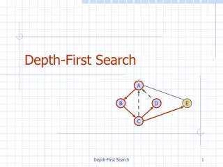
Graph Algorithms Using Depth First Search
Graph Algorithms Using Depth First Search. Analysis of Algorithms Week 8, Lecture 1. Prepared by John Reif, Ph.D. Distinguished Professor of Computer Science Duke University. Graph Algorithms Using Depth First Search. Graph Definitions DFS of Graphs Biconnected Components


Graph Algorithms Using Depth First Search
E N D
Presentation Transcript
Graph Algorithms Using Depth First Search Analysis of Algorithms Week 8, Lecture 1 Prepared by John Reif, Ph.D. Distinguished Professor of Computer Science Duke University
Graph Algorithms Using Depth First Search • Graph Definitions • DFS of Graphs • Biconnected Components • DFS of Digraphs • Strongly Connected Components
Readings on Graph Algorithms Using Depth First Search • Reading Selection: • CLR, Chapter 22
Graph Terminology • GraphG=(V,E) • Vertex setV • Edge setE pairs of vertices which are adjacent
u v Directed and Undirected Graphs • G directed • G undirected u v
Proper Graphs and Subgraphs • Proper graph: • No loops • No multi-edges • SubgraphG‘ of G G‘ = (V‘, E‘) where V‘ is a subset of V, E‘ is a subset of E
e1 e2 ek Vo V2 Vk-1 Vk V1 Paths in Graphs • Path p P is a sequence of vertices v0, v1, …, vk where for i=1,…k, vi-1 is adjacent to vi Equivalently, p is a sequence of edges e1, …, ek where for i = 2,…k edges ei-1, ei share a vertex
V2 Vk-1 Vk = Vo V1 Simple Paths and Cycles • Simple path no edge or vertex repeated, except possibly vo = vk • Cycle a path p with vo = vk where k>1
(or G is single edge) Biconnected Undirected Graphs
1 2 3 4 Size of a Graph • Graph G = (V,E) n = |V| = # vertices m = |E| = # edges size of G is n+m
Representing a Graph by an Adjacency Matrix • Adjacency Matrix A
1 2 3 1 3 2 3 1 2 4 4 3 Adjacency List Representation of a Graph • Adjacency ListsAdj (1),…,Adj (n) Adj(v) = list of vertices adjacent to v space cost O(n+m)
Definition of an Undirected Tree • Tree T is graph with unique path between every pair of vertices n = # vertices n-1 = # edges • Forest • set of trees
r Definition of a Directed Tree • Directed Tree T is digraph with distinguished vertex root r such that each vertex reachable from r by a unique path Family Relationships: - ancestors - descendants - parent - child - siblings leaves have no proper descendants
A B C D F E H I An Ordered Tree • Ordered Tree • is a directed tree with siblings ordered
A B C D F E H I Preorder Tree Traversal • Preorder A,B,C,D,E,F,H,I [1] root (order vertices as pushed on stack) [2] preorder left subtree [3] preorder right subtree
A B C D F E H I Postorder Tree Traversal • Postorder B,E,D,H,I,F,C,A [1] postorder left subtree [2] postorder right subtree [3] root (order vertices as popped off stack)
Spanning Tree and Forest of a Graph • T is a spanning tree of graph G if (1) T is a directed tree with the same vertex set as G (2) each edge of T is a directed version of an edge of G • Spanning Forest: forest of spanning trees of connected components of G
root 1 back edge tree edge 2 5 9 12 6 3 8 10 11 7 4 cross edge Example Spanning Tree of a Graph
Classification of Edges of G with Spanning Tree T • An edge (u,v) of T is tree edge • An edge (u,v) of G-T is back edge if u is a descendent or ancestor of v. • Else (u,v) is a cross edge
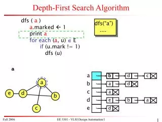
Tarjan’s Depth First Search Algorithm • We assume a RAM machine model • Algorithm Depth First Search
Time Cost of Depth First Search Algorithm on a RAM • Input size n = |V|, m = |E| • Theorem Depth First Search takes total time cost O(n+m) • Proof can associate with each edge and vertex a constant number of operations.
G 1 2 5 1 T 6 3 8 2 5 7 6 8 3 4 4 7 Classification of Edges of G via DFS Spanning Tree T
Classification of Edges of G via DFS Spanning Tree T • Edge notation induced by • Depth First Search Tree T
Classification of Edges of G via DFS Spanning Tree T (cont’d) • Note DFS tree T has no cross edges will number vertices by order visited in DFS (preorder of T)
W * v Dv u Verifying Vertices are Descendants via Preordering of Tree • Suppose we preorder number a Tree T Let Dv = # of descendants of v • Lemma u is descendant of v iff v u v + Dv
Testing for Proper Ancestors via Preordering • Lemma If u is descendant of v and (u,w) is back edge s.t. w v then w is a proper ancestor of v
Low Values • For each vertex v, define low(v) = min ( {v} {w | v - - - w} ) • Can prove by induction: Lemma can be computed during DFS in postorder. *
v[low(v)] 1[1] 5[1] 2[2] 8[1] 3[2] 6[5] 4[2] Number vertices by DFS number 7[5] Graph with DFS Numbering and Low Values in Brackets
Biconnected Components • G is Biconnected iff either (1) G is a single edge, or (2) for each triple of vertices u,v,w
1 1 2 1 G 5 2 8 5 3 2 6 8 5 3 4 6 7 4 7 Example of Biconnected Components of Graph G • Maximal subgraphs of G which are biconnected.
1 G 2 5 6 8 3 4 7 Biconnected Components Meet at Articulation Points • The intersection of two biconnected components consists of at most one vertex called an Articulation Point. • Example: 1,2,5 are articulation points
Discovery of Biconnected Components via Articulation Points • If can find articulation points then can compute biconnected components: Algorithm: • During DFS, use auxiliary stack to store visited edges. • Each time we complete the DFS of a tree child of an articulation point, pop all stacked edges • currently in stack • These popped off edges form a biconnected component
Characterization of an Articulation Point • Theorem a is an articulation point iff either (1) a is root with 2 tree children or (2) a is not root but a has a tree child v with low (v) a (note easy to check given low computation)
Proof of Characterization of an Articulation Point • Proof The conditions are sufficient since any a-avoiding path from v remains in the subtree Tv rooted at v, if v is a child of a • To show condition necessary, assume a is an articulation point.
Characterization of an Articulation Point (cont’d) • Case (1) If a is a root and is articulation point, a must have 2 tree edges to two distinct biconnected components. • Case(2) If a is not root, consider graph G - {a} which must have a connected component C consisting of only descendants of a, and with no backedge from C to an ancestor of v. Hence a has a tree child v in C and low (v) a
root Articulation Point a is not the root no back edges a v subtree Tv C Proof of Characterization of an Articulation Point (cont’d) • Case (2)
Computing Biconnected Components • Theorem The Biconnected Components of G = (V,E) can be computed in time O(|V|+|E|) using a RAM • Proof idea • Use characterization of Bicoconnected components via articulation points • Identify these articulation points dynamically during depth first search • Use a secondary stack to store the edges of the biconnected components as they are visited • When an articulation point is discovered , pop the edges of this stack off to output a biconnected component
Biconnected Components Algorithm [0] initialize a STACK to empty During a DFS traversal do [1] add visited edge to STACK [2] compute low of visited vertex v using Lemma [3] test if v is an articulation point [4] if so, for each u children (v) in order where low (u) > v do Pop all edges in STACK upto and including tree edge (v,u) Output popped edges as a biconnected component of G od
Time Bounds of Biconnected Components Algorithm • Time Bounds: Each edge and vertex can be associated with 0(1) operations. So time O(|V|+|E|).
G = (V,E) 8 i = DFS number 1 forward i 7 v 2 cycle i = postorder = order vertex popped off DFS stack 5 3 cycle 4 6 7 4 8 cross cross 5 2 edge set E partitioned cross 1 6 Depth First Search in a Directed Graph • Depth first search tree T of Directed Graph
Classification of Directed Edge (u, v) via DFS Spanning Tree T • Tree edge • Cycle edge • Forward edge • Cross edge
Topological Order of Acyclic Directed Graph • Digraph G = (V,E) is acyclic if it has no cycles
Characterization of an Acyclic Digraph • Proof Case (1): • Suppose (u,v) E is a cycle edge, so v → u. • But let e1,…ek be the tree edges from v to u. • Then (u,v), e1,…ek is a cycle. *
Characterization of an Acyclic Digraph (cont’d) Case (2): • Suppose G has no a cycle edge • Then order vertices in postorder of DFS spanning forest (i.e. in order vertices are popped off DFS stack). • This is a reverse topological order of G. • So, G can have no cycles. Note: Gives an O(|V|+|E|) algorithm for computing Topological Ordering of an acyclic graph G = (V,E)
Strong Components of Directed Graph • Strong Component • Collapsed Graph G* derived by collapsing each strong component into a single vertex. note: G* is acyclic.
8 Directed Graph with Strong Components Circled 1 4 Directed Graph G = (V,E) 2 5 3 6 7