Bethe-Bloch Theory in Proton Stopping Power Calculation
290 likes | 401 Views
Learn about Bethe-Bloch theory for proton stopping power in detail, including the effects of different materials and energy levels. Explore the complexities and simplifications of the theory for clinical applications.

Bethe-Bloch Theory in Proton Stopping Power Calculation
E N D
Presentation Transcript
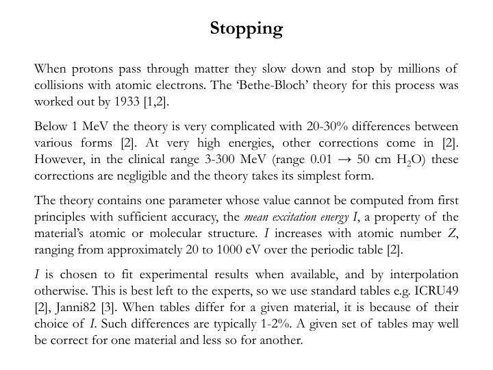
Stopping When protons pass through matter they slow down and stop by millions ofcollisions with atomic electrons. The ‘Bethe-Bloch’ theory for this process was worked out by 1933 [1,2]. Below 1 MeV the theory is very complicated with 20-30% differences between various forms [2]. At very high energies, other corrections come in [2]. However, in the clinical range 3-300 MeV (range 0.01 → 50 cm H2O) these corrections are negligible and the theory takes its simplest form. The theory contains one parameter whose value cannot be computed from first principles with sufficient accuracy, the mean excitation energyI, a property of the material’s atomic or molecular structure. I increases with atomic number Z, ranging from approximately 20 to 1000 eV over the periodic table [2]. I is chosen to fit experimental results when available, and by interpolation otherwise. This is best left to the experts, so we use standard tables e.g. ICRU49 [2], Janni82 [3]. When tables differ for a given material, it is because of their choice of I. Such differences are typically 1-2%. A given set of tables may well be correct for one material and less so for another.
In its simplest form the theory fits on one page. Bethe’s formula for the electronic mass stopping power is Z, A are the atomic number and relative atomic mass of the target atom, z is the charge number of the projectile and β = v/c. The first term is a constant: L(β)is called the stopping number. If all four corrections to the Bethe formula are ignored (OK at therapy energies) one finds where Wm is the largest possible energy loss in a single collision with a free electron and I is the mean excitation energy of the medium. Wm is given by but at therapy energies the factor in square brackets can be set to 1. Finally, it is convenient to know that
Mean Excitation Energy I This graph from ICRU 49 [2] shows the dependence of I on atomic number Z. Irregularities in I/Z vs. Z are caused by atomic shell structure. It’s obvious that interpolating I accurately between measured values (from range or stopping power measurements) is not easy.
Mixtures, Compounds and Molecules Mixtures obey the Bragg additivity rule, which is easily derived by assuming the absorber to be composed of several discrete sheets: Compounds and molecules are more complicated because I is affected by chemical bonding. Water turns out to be a particularly difficult case, which is unfortunate. R (160, water) = 17.648 g/cm2 (ICRU49) = 17.806 (+0.9%) (Janni82) It seems that the Janni82 value is better (Moyers et al., Med. Phys. 34 (2007) 1952-1966)
Range Proton range is the integral of inverse stopping power. The proton enters at T and stops when the kinetic energy is 0 . Sometimes it is convenient to write the integral in a universal form: Strictly speaking, the integrals we have written down are the proton pathlength. However, protons scatter very little so for practical purposes the pathlength equals the projected range. Experimentally, the computed range is interpreted as the depth by which half the protons have stopped, is written r0, and is called the mean projected range or just range.
The Power Law The graph shows the integrand (second formula, previous page) in its universal form where it depends only on T/mc2. If that were a straight line, the integral would be (T/mc2 )2. Since it increases slower than linearly, the power is less than 2. For water in the clinical energy range, R ≈ a T 1.78 . For other materials the exponent is slightly different. The power law approximation is common in the literature, but we normally use a more accurate relation, described later.
Range Straggling Range straggling refers to the spread in proton ranges (even in a monoenergetic beam) because energy loss is a statistical process that occurs in discrete steps. The full theory is complicated: see Janni [3], who also gives tables. The spread can be characterized by a Gaussian with an rms value σS , which is nearly proportional to r0(see graph). This nearly material-independent behavior has important consequences: it means we can assume the Bragg peak in H2O has a constant shape even if some stopping occurred in Pb.
Range-Energy for Other Particles Because the range-energy relation depends only on particle speed it is possible to write down scaling rules to find it for other particles if it is known for protons. The example shows the case for αparticles. The range of a 200 MeV α equals the range of a 50 MeV proton (1/4 the energy).
Measuring Range Having talked about how to predict range, let’s see how we measure it. The simplest arrangement (left) consists of a beam monitor and a stack of known degraders placed in front of a Faraday cup. This measures (in accordance with the definition of range) the number of surviving protons (not the dose!) as a function of projected depth in CH2 or whatever (aluminum is also good). Data (right) show a gradual falloff as protons succumb to nuclear reactions: charged secondaries will mostly miss the FC because of the distance. r0 is the x value of the halfway point measured from the corner (y ≈ 0.37) not the entrance (y ≈ 0.53). The open circles were taken with a different FC with the CH2 much closer to the charge collector.
Measuring Range (continued) It may not be convenient to use a Faraday cup. Frequently all we have is a small dosimeter (rather than a fluence meter) and a water tank. In that case we’ll measure a depth-dose distribution, that is, a Bragg peak (BP) (bottom frame). That clearly tells us something about the range, but what exact point on the BP equals r0? The answer was first found by Andy Koehler using a graphical method of calculation: r0 = d80, the distal 80% point of the BP. This has since been confirmed by several others. The result is purely numerical (not an analytic ‘proof’) so the 80 is not exactly 80, but close enough. A number of BP’s taken at the same mean energy but with different energy spreads will intersect at d80, making it a good physics benchmark. Clinically,we are more likely to be interested in d90.
d80 versus d90 In designing clinical setups we must keep track of what the clinicians actually want and how it relates to the range d80. Our programs are forever computing depths and then correcting for the difference between d80 and (say) d90. That depends on energy and energy spread, and must be measured. The data shown are from the Burr Center.
Interpolating Range-Energy Tables As we already know from the power-law approximation, the range-energy relation is nearly a straight line in a log-log presentation (top). Therefore we use cubic spline interpolation in log(R) vs. log(T) to find intermediate values. That is equivalent to using a variable-power law. It is accurate to ≈ 0.1% over the clinical range 3-300 MeV (bottom), even if we only enter 13 table values. This is how LOOKUP does it.
Program and Data File Examples Typical Fortran fragment : Fragment of JANNI82.RET :
Typical Problem Find the energy out of 5 g/cm2 Lexan for 160 Mev incident protons. R1 R2 T1 160 MeV M1 = ‘Lexan’ G1 = 5 g/cm2 We write this problem in shorthand
Solution Exact method using range: Approximate method using stopping power: Summary:
Fortran Implementation Exact method : In Fortran all that can be written : We never use the approximate method in programs. The slight gain in speed is not worth the extra bookeeping.
Water Equivalence In proton therapy two degraders are equivalent if the energy loss is the same. The thickness of water tW that gives the same energy loss as a thickness tM of some other material, at incident energy Ei , can be found exactly (LOOKUP/WATEREQ): However, if we do that calculation for the same lead degrader at two different energies we’ll get different answers because the stopping power ratio depends on energy: the curves for Pb and water are not quite parallel. The 0.62 cm Pb in the second scatterer of the Burr Center nozzle is equivalent to 3.556 cm H2O at 200 MeV and 3.355 at 70 Mev. The 2 mm difference is just enough to be troublesome. The plastic/water ratio is independent of energy so water equivalence of plastic is a safer concept. If you really need an accurate water equivalent it’s better to measure it.
ΔT ΔT′ T T′ Energy Spread of Degraded Beams Suppose you are managing a non-clinical user program where you supply various energies by degrading the beam. The customer wants to know the energy spread of the degraded beam. Andy Koehler found that as a consequence of the nonlinearity of the range-energy relation. The proof is easy. The formula is only approximate. If T′ is very small its distribution becomes skewed (asymmetric).
A Related Issue unknown energy distribution known energy distribution A B A d Suppose we have a dosimeter (plane parallel ion chamber) at some depth in a water tank. It responds to the mix of energies at that depth. It signal will change very little if we remove surrounding volumes of water A and distal volume B: side- and back-scattering effects are negligible in most cases for protons. That has far reaching consequences. It means the energy distribution inside a water tank is the same as that behind the equivalent water column. We can measure a Bragg peak either with a water tank or a water column; more important, we can measure the Bragg peak in solids behind a stack of degraders. All this would be much less true for electrons, where backscattering can be significant.
Proof of ΔT′/ΔT = (S/ρ)′/(S/ρ) For any ΔT (MeV) and a corresponding ΔR (g/cm2), by definition T1 T1′ T2 T2′ For the incident energies this reads T1′ T1 R(T1′) and for the outgoing energies it reads R(T1) ΔR But the LH sides are just two different expression for ΔR (see sketch at left). So the RH sides are equal and Andy’s formula follows. T2 T2′ R(T2′) R(T2)
Another Way of Looking at It As protons penetrate a degrader their energy spread increases. To show why, we have drawn the hypothetical range-energy curves for monoenergetic 152 and 160 MeV protons in water ignoring range straggling. The dispersion in width with depth is due solely to the nonlinear range-energy relation!
Energy Degraders Used With Cyclotrons Cyclotron-based therapy facilities use degraders to change the beam energy because variable-energy cyclotrons are very expensive and energy changes are very slow. The resulting increase in energy and angular spread is pared away by slits but a lot of beam is lost in the process.
NaI SCINTILLATOR DEGRADER TO PULSE-HEIGHT ANALYZER Measuring ΔT′/ΔT = (S/ρ)′/(S/ρ) From Cascio et al. ‘Measurements of the energy spectrum of degraded beams at NPTC,’ Proc. IEEE Radiation Effects Data Workshop (2004) 151. The energy spectrum was measured with a NaI scintillation spectrometer at a given setting of the NPTC momentum slits. The long tail to the left of the peak is an artifact from nuclear reactions in the NaI crystal; a magnetic spectrometer would be better.
Measuring ΔT′/ΔT = (S/ρ)′/(S/ρ) (final) From Cascio et al. The full prediction of observed ΔT′ is more complicated than the simple formula. One must include detector resolution and the fact that some energy width would develop from straggling even if the incident energy spread were zero.
Funny Things Can Happen This eye beam degrader (originally clear Lexan) was in a strongly focused beam for years. Eventually the energy width of the output beam increased. Watch out for this!
Summary The range-energy relation for a material depends on an empirical parameter I. Since I is hard to choose, we leave it to the experts and use tables, which may differ by 1-2%. The proton range r0 is defined as the depth where 50% of the protons have stopped, not counting those that suffer nuclear reactions. Ideally it should be measured with a fluence meter. If a dosimeter must be used (Bragg peak) use r0 = d80 . Range straggling is a nearly constant percentage of range and nearly the same for all materials. That makes the shape of the Bragg peak nearly independent of the stopping material, an extremely important result for the designer. The range-energy relation in a given material is approximately described by the power law r0 ≈ A TB . A and B depend on the material. B is always a little less than 2. In practice, though, we find ranges by cubic spline interpolation of log(R) vs. log(T). We solve degrader problems by manipulating range-energy relations directly. The more obvious dE/dx method is seriously wrong for thick degraders. Usually, we will solve design problems by working with range, pullback etc. In other words, we rarely need to know the energy or energy spread in the beam. If we do, we can use ΔT′ ≈ ΔT × (S/ρ)′/(S/ρ) to estimate it. Severe radiation damage can affect a degrader, causing a larger output energy spread. N.B. we can use range-energy tables for most design work but because of the ~3mm/30cm uncertainty we must never use them to determine treatment depth in a patient. Instead, we must use measured depth in water or measured water equivalents.