Download
1 / 66
680 likes | 872 Views
Chapter 3. Algorithms for Query Processing and Optimization. Chapter Outline. Introduction to Query Processing Translating SQL Queries into Relational Algebra Algorithms for External Sorting Algorithms for SELECT and JOIN Operations Algorithms for PROJECT and SET Operations

E N D
Chapter 3 Algorithms for Query Processing and Optimization
Chapter Outline • Introduction to Query Processing • Translating SQL Queries into Relational Algebra • Algorithms for External Sorting • Algorithms for SELECT and JOIN Operations • Algorithms for PROJECT and SET Operations • Implementing Aggregate Operations and Outer Joins • Combining Operations using Pipelining • Using Heuristics in Query Optimization • Using Selectivity and Cost Estimates in Query Optimization • Overview of Query Optimization in Oracle • Semantic Query Optimization
Introduction to Query Processing • Query optimization: the process of choosing a suitable execution strategy for processing a query. • Two internal representations of a query • – Query Tree • – Query Graph
Translating SQL Queries into Relational Algebra (1) • Query block: the basic unit that can be translated into the algebraic operators and optimized. • A query block contains a single SELECT-FROM-WHERE expression, as well as GROUP BY and HAVING clause if these are part of the block. • Nested queries within a query are identified as separate query blocks. • Aggregate operators in SQL must be included in the extended algebra.
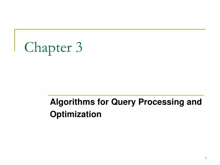
Algorithms for External Sorting (1) • External sorting : refers to sorting algorithms that are suitable for large files of records stored on disk that do not fit entirely in main memory, such as most database files. • Sort-Merge strategy : starts by sorting small subfiles (runs ) of the main file and then merges the sorted runs, creating larger sorted subfiles that are merged in turn. – Sorting phase: nR = (b/nB) – Merging phase: dM = Min(nB-1, nR); nP= (logdM(nR)) nR: number of initial runs; b: number of file blocks; nB: available buffer space; dM: degree of merging; nP: number of passes.
a 19 d 31 a 19 g 24 g 24 b 14 a 14 a 19 c 33 a 19 d 31 b 14 d 31 b 14 c 33 c 33 e 16 c 33 b 14 e 16 g 24 d 7 e 16 d 21 r 16 d 31 a 14 d 31 d 21 m 3 d 7 e 16 m 3 r 16 d 21 g 24 p 2 m 3 m 3 d 7 a 14 p 2 p 2 a 14 d 17 r 16 r 16 p 2 Buffer-size = 3 Tạo run trộn pass-1 trộn pass-2
Algorithms for External Sorting (2) set i 1, j b; /* size of the file in blocks */ k nB; /* size of buffer in blocks */ m (j/k); {Sort phase} while (i<= m) do { read next k blocks of the file into the buffer or if there are less than k blocks remaining, then read in the remaining blocks; sort the records in the buffer and write as a temporary subfile; i i+1; }
/*Merge phase: merge subfiles until only 1 remains */ set i 1; p logk-1m; { p is the number of passes for the merging phase } j m; while (i<= p) do { n 1; q (j/(k-1); while ( n <= q) do { read next k-1 subfiles or remaining subfiles (from previous pass) one block at a time merge and write as new subfile one block at a time; n n+1; } j q; i i+1; }
Algorithms for SELECT and JOIN Operations (1) Implementing the SELECT Operation: Examples: • (OP1): σSSN='123456789'(EMPLOYEE) • (OP2): σDNUMBER>5(DEPARTMENT) • (OP3): σDNO=5(EMPLOYEE) • (OP4): σDNO=5 AND SALARY>30000 AND SEX=F(EMPLOYEE) • (OP5): σESSN=123456789 AND PNO=10(WORKS_ON)
Algorithms for SELECT and JOIN (2) Implementing the SELECT Operation (cont.): Search Methods for Simple Selection: • S1. Linear search (brute force): Retrieve every record in the file, and test whether its attribute values satisfy the selection condition. • S2. Binary search : If the selection condition involves an equality comparison on a key attribute on which the file is ordered, binary search (which is more efficient than linear search) can be used. (See OP1). • S3. Using a primary index or hash key to retrieve a single record: If the selection condition involves an equality comparison on a key attribute with a primary index (or a hash key), use the primary index (or the hash key) to retrieve the record.
Algorithms for SELECT and JOIN Operations (3) Implementing the SELECT Operation (cont.): Search Methods for Simple Selection: • S4. Using a primary index to retrieve multiple records: If the comparison condition is >, ≥ , <, or ≤ on a key field with a primary index, use the index to find the record satisfying the corresponding equality condition, then retrieve all subsequent records in the (ordered) file. • S5. Using a clustering index to retrieve multiple records: If the selection condition involves an equality comparison on a non-key attribute with a clustering index, use the clustering index to retrieve all the records satisfying the selection condition.
Algorithms for SELECT and JOIN Operations (4) Implementing the SELECT Operation (cont.): Search Methods for Simple Selection: • S6. Using a secondary (B+-tree) index : On an equality comparison, this search method can be used to retrieve a single record if the indexing field has unique values (is a key) or to retrieve multiple records if the indexing field is not a key. In addition, it can be used to retrieve records on conditions involving >,>=, <, or <=. (FOR RANGE QUERIES )
Algorithms for SELECT and JOIN (5) Implementing the SELECT Operation (cont.): Search Methods for Complex Selection: • S7. Conjunctive selection : If an attribute involved in any single simple condition in the conjunctive condition has an access path that permits the use of one of the methods S2 to S6, use that condition to retrieve the records and then check whether each retrieved record satisfies the remaining simple conditions in the conjunctive condition. • S8. Conjunctive selection using a composite index: If two or more attributes are involved in equality conditions in the conjunctive condition and a composite index (or hash structure) exists on the combined field, we can use the index directly.
Algorithms for SELECT and JOIN (6) Implementing the SELECT Operation (cont.): Search Methods for Complex Selection: • S9. Conjunctive selection by intersection of record pointers : This method is possible if secondary indexes are available on all (or some of) the fields involved in equality comparison conditions in the conjunctive condition and if the indexes include record pointers (rather than block pointers). Each index can be used to retrieve the record pointers that satisfy the individual condition. The intersection of these sets of record pointers gives the record pointers that satisfy the conjunctive condition, which are then used to retrieve those records directly. If only some of the conditions have secondary indexes, each retrieved record is further tested to determine whether it satisfies the remaining conditions.
Algorithms for SELECT and JOIN Operations (7) Implementing the SELECT Operation (cont.): • Whenever a single condition specifies the selection, we can only check whether an access path exists on the attribute involved in that condition. If an access path exists, the method corresponding to that access path is used; otherwise, the “brute force” linear search approach of method S1 is used. (See OP1, OP2 and OP3) • For conjunctive selection conditions, whenever more than one of the attributes involved in the conditions have an access path, query optimization should be done to choose the access path that retrieves the fewest records in the most efficient way. • Disjunctive selection conditions
Algorithms for SELECT and JOIN Operations (8) Implementing the JOIN Operation: • Join (EQUIJOIN, NATURAL JOIN) – two–way join: a join on two files e.g. R A=B S – multi-way joins: joins involving more than two files. e.g. R A=B S C=DT • Examples (OP6): EMPLOYEE DNO=DNUMBERDEPARTMENT (OP7): DEPARTMENT MGRSSN=SSNEMPLOYEE
Algorithms for SELECT and JOIN Operations (9) Implementing the JOIN Operation (cont.): Methods for implementing joins: • J1. Nested-loop join (brute force): For each record t in R (outer loop), retrieve every record s from S (inner loop) and test whether the two records satisfy the join condition t[A] = s[B]. • J2. Single-loop join (Using an access structure to retrieve the matching records): If an index (or hash key) exists for one of the two join attributes — say, B of S — retrieve each record t in R, one at a time, and then use the access structure to retrieve directly all matching records s from S that satisfy s[B] = t[A].
Algorithms for SELECT and JOIN Operations (10) Implementing the JOIN Operation (cont.): Methods for implementing joins: • J3. Sort-merge join: If the records of R and S are physically sorted (ordered) by value of the join attributes A and B, respectively, we can implement the join in the most efficient way possible. Both files are scanned in order of the join attributes, matching the records that have the same values for A and B. In this method, the records of each file are scanned only once each for matching with the other file—unless both A and B are non-key attributes, in which case the method needs to be modified slightly.
C A 5 6 9 10 17 20 BD 4 6 6 10 17 18 Assume that A is a key of R. Initially, two pointers are used to point to the two tuples of the two relations that have the smallest values of the two joining attributes.
Algorithms for SELECT and JOIN Operations (11) Implementing the JOIN Operation (cont.): Methods for implementing joins: • J4. Hash-join: The records of files R and S are both hashed to the same hash file, using the same hashing function on the join attributes A of R and B of S as hash keys. A single pass through the file with fewer records (say, R) hashes its records to the hash file buckets. A single pass through the other file (S) then hashes each of its records to the appropriate bucket, where the record is combined with all matching records from R.
Algorithms for SELECT and JOIN Operations (12) (a) sort the tuples in R on attribute A; /* assume R has n tuples */ sort the tuples in S on attribute B; /* assumeS has m tuples */ set i 1, j 1; while (i ≤ n) and (j ≤ m) do { if R(i)[A] > S[j][B] then set j j + 1 elseif R(i)[A] < S[j][B] then set i i + 1 else { /* output a matched tuple */ output the combined tupe <R(i), S(j)> to T; /* output other tuples that match R(i), if any */ set l j + 1 ; while ( l ≤ m) and (R(i)[A] = S[l][B]) do { output the combined tuple <R(i), S[l]> to T; set l l + 1 } /* output other tuples that match S(j), if any */ set k i+1 while ( k ≤ n) and (R(k)[A] = S[j][B]) do { output the combined tuple <R(k), S[j]> to T; set k k + 1 } set i i+1, j j+1; } } (a) Implementing T R A=B S
Implementing T ∏<attribute list>(R) (b) create a tuple t[<attribute list>] in T’ for each tuple t in R; /* T’ contains the projection result before duplicate elimination */ if <attribute list> includes a key of R then T T’ else { sort the tuples in T’; set i 1, j 2; while i ≤ n do { output the tuple T’[i] to T; while T’[i] = T[j] and j≤ n do j j+1; set i j, j i+1; } } /* T’ contains the projection result after duplicate elimination */ b) Implementing T ∏<attribute list>(R)
Algorithms for PROJECT and SET Operations (1) • Algorithm for PROJECT operations π<attribute list>(R) (Figure 15.3b) • If <attribute list> has a key of relation R, extract all tuples from R with only the values for the attributes in <attribute list>. • If <attribute list> does NOT include a key of relation R, duplicated tuples must be removed from the results. • Methods to remove duplicate tuples: • 1. Sorting • 2. Hashing
Algorithms for PROJECT and SET Operations (2) Algorithm for SET operations • Set operations : UNION, INTERSECTION, SET DIFFERENCE and CARTESIAN PRODUCT. • CARTESIAN PRODUCT of relations R and S include all possible combinations of records from R and S. The attribute of the result include all attributes of R and S. • Cost analysis of CARTESIAN PRODUCT If R has n records and j attributes and S has m records and k attributes, the result relation will have n*m records and j+k attributes. • CARTESIAN PRODUCT operation is very expensive and should be avoided if possible.
Algorithms for PROJECT and SET Operations (3) • Algorithm for SET operations (Cont.) • UNION (See Figure 15.3c) • 1. Sort the two relations on the same attributes. • 2. Scan and merge both sorted files concurrently, whenever the same tuple exists in both relations, only one is kept in the merged results. • INTERSECTION (See Figure 15.3d) • 1. Sort the two relations on the same attributes. • 2. Scan and merge both sorted files concurrently, keep in the merged results only those tuples that appear in both relations. • SET DIFFERENCE R-S (See Figure 15.3e)(keep in the merged results only those tuples that appear in relation R but not in relation S.)
Union: T R S (c) sort the tuples in R and S using the same unique sort attributes; set i 1, j 1; while (i ≤ n) and (j ≤ m) do { if R(i) > S(j) then { output S(j) to T; set j j+1 } elseif R(i) < S(j) then { output R(i) to T; set i i+1 } else set j j+1 /* R(i) = S(j), so we skip one of the duplicate tuples */ } if (i ≤ n) then add tuples R(i) to R(n) to T; if (j ≤ m) then add tuples S(i) to S(m) to T;
Intersection T R S (d) sort the tuples in R and S using the same unique sort attributes; set i 1, j 1; while (i ≤ n) and (j ≤ m) do { if R(i) > S(j) then set j j+1 elseif R(i) < S(j) then set i i+1 else { output R(i) to T; /* R(i) = S(j), so we skip one of the duplicate tuples */ set i i+1, j j+1 } }
Difference T R S (e) sort the tuples in R and S using the same unique sort attributes; set i 1, j 1; while (i ≤ n) and (j ≤ m) do { if R(i) > S(j) then set j j+1 elseif R(i) < S(j) then { output R(i) to T; /* R(i) has no matching S(j), so output R(i) */ set i i+1 } else set i i+1, j j+1 } if (i ≤ n) then add tuples R(i) to R(n) to T;
5. Implementing Aggregate Operations and Outer Joins (1) Implementing Aggregate Operations: • Aggregate operators : MIN, MAX, SUM, COUNT and AVG • Options to implement aggregate operators: • Table Scan • Index • Example • SELECT MAX(SALARY) FROM EMPLOYEE; • If an (ascending) index on SALARY exists for the employee relation, then the optimizer could decide on traversing the index for the largest value, which would entail following the right most pointer in each index node from the root to a leaf.
Implementing Aggregate Operations and Outer Joins (2) • Implementing Aggregate Operations (cont.): • SUM, COUNT and AVG • 1. For a dense index (each record has one index entry): apply the associated computation to the values in the index. • 2. For a non-dense index: actual number of records associated with each index entry must be accounted for • With GROUP BY: the aggregate operator must be applied separately to each group of tuples. • 1. Use sorting or hashing on the group attributes to partition the file into the appropriate groups; • 2. Computes the aggregate function for the tuples in each group. • What if we have Clustering index on the grouping attributes?
Implementing Aggregate Operations and Outer Joins (3) • Implementing Outer Join: • Outer Join Operators : LEFT OUTER JOIN, RIGHT OUTER JOIN and FULL OUTER JOIN. • The full outer join produces a result which is equivalent to the union of the results of the left and right outer joins. • Example: SELECT FNAME, DNAME FROM ( EMPLOYEE LEFT OUTER JOIN DEPARTMENT ON DNO = DNUMBER); • Note: The result of this query is a table of employee names and their associated departments. It is similar to a regular join result, with the exception that if an employee does not have an associated department, the employee's name will still appear in the resulting table, although the department name would be indicated as null.
Implementing Aggregate Operations and Outer Joins (4) • Implementing Outer Join (cont.): • Modifying Join Algorithms:Nested Loop or Sort-Merge joins can be modified to implement outer join. e.g., for left outer join, use the left relation as outer relation and construct result from every tuple in the left relation. If there is a match, the concatenated tuple is saved in the result. However, if an outer tuple does not match, then the tuple is still included in the result but is padded with a null value(s).
Implementing Aggregate Operations and Outer Joins (5) • Implementing Outer Join (cont.): Executing a combination of relational algebra operators. Implement the previous left outer join example 1. {Compute the JOIN of the EMPLOYEE and DEPARTMENT tables} TEMP1 FNAME,DNAME(EMPLOYEE DNO=DNUMBER DEPARTMENT) 2. {Find the EMPLOYEEs that do not appear in the JOIN} TEMP2 FNAME(EMPLOYEE) - FNAME(Temp1) 3. {Pad each tuple in TEMP2 with a null DNAME field} TEMP2 TEMP2 x 'null' 4. {UNION the temporary tables to produce the LEFT OUTER JOIN result} RESULT TEMP1 TEMP2 The cost of the outer join, as computed above, would include the cost of the associated steps (i.e., join, projections and union).
6. Combining Operations using Pipelining (1) • Motivation • – A query is mapped into a sequence of operations. • – Each execution of an operation produces a temporary result. • – Generating and saving temporary files on disk is time consuming and expensive. • Alternative: • – Avoid constructing temporary results as much as possible. • – Pipeline the data through multiple operations - pass the result of a previous operator to the next without waiting to complete the previous operation.
Combining Operations using Pipelining (2) • Example: For a 2-way join, combine the 2 selections on the input and one projection on the output with the Join. • Dynamic generation of code to allow for multiple operations to be pipelined. • Results of a select operation are fed in a " Pipeline " to the join algorithm. • Also known as stream-based processing.
Using Heuristics in Query Optimization(1) Process for heuristics optimization • 1. The parser of a high-level query generates an initial internal representation; • 2. Apply heuristics rules to optimize the internal representation. • 3. A query execution plan is generated to execute groups of operations based on the access paths available on the files involved in the query. • The main heuristic is to apply first the operations that reduce the size of intermediate results. E.g., Apply SELECT and PROJECT operations before applying the JOIN or other binary operations.
Using Heuristics in Query Optimization (2) • Query tree : a tree data structure that corresponds to a relational algebra expression. It represents the input relations of the query as leaf nodes of the tree, and represents the relational algebra operations as internal nodes. • An execution of the query tree consists of executing an internal node operation whenever its operands are available and then replacing that internal node by the relation that results from executing the operation. • Query graph : a graph data structure that corresponds to a relational calculus expression. It does not indicate an order on which operations to perform first. There is only a single graph corresponding to each query.
Using Heuristics in Query Optimization (3) • Example: For every project located in ‘Stafford’, retrieve the project number, the controlling department number and the department manager’s last name, address and birthdate. • Relation algebra : PNUMBER, DNUM, LNAME, ADDRESS, BDATE(((σPLOCATION=‘STAFFORD’(PROJECT)) DNUM=DNUMBER (DEPARTMENT)) MGRSSN=SSN (EMPLOYEE)) • SQL query : Q2: SELECT P.NUMBER,P.DNUM,E.LNAME, E.ADDRESS, E.BDATE FROM PROJECT AS P,DEPARTMENT AS D, EMPLOYEE AS E WHERE P.DNUM=D.DNUMBER AND D.MGRSSN=E.SSN AND P.PLOCATION=‘STAFFORD’;
Using Heuristics in Query Optimization (6) Heuristic Optimization of Query Trees : • The same query could correspond to many different relational algebra expressions — and hence many different query trees. • The task of heuristic optimization of query trees is to find a final query tree that is efficient to execute. • Example : Q: SELECT LNAME FROM EMPLOYEE, WORKS_ON,PROJECT WHERE PNAME = ‘AQUARIUS’ AND PNMUBER=PNO AND ESSN=SSN AND BDATE > ‘1957-12-31’;
Step in converting a query during heuristic optimization. Initial query tree
Apply more restrictive SELECT operation first Replacing Cartesian Product and Select with Join operation.
Using Heuristics in Query Optimization (10) General Transformation Rules for Relational Algebra Operations: 1. Cascade of σ : A conjunctive selection condition can be broken up into a cascade (sequence) of individual selection operations: σc1 AND c2 AND ... AND cn(R) = σc1(σc2(...( σcn(R))...) ) 2.Commutativity of σ : The σ operation is commutative: σc1(σc2(R)) = σc2(σc1(R)) • 3. Cascade of π : In a cascade (sequence) of π operations, all but the last one can be ignored: πList1(π List2(...( πListn (R))...) ) = π List1(R) • 4. Commuting σ with π : If the selection condition c involves only the attributes A1, ..., An in the projection list, the two operations can be commuted: πA1, A2,., An(σc(R)) = σc(πA1, A2,., An (R))
Using Heuristics in Query Optimization (11) • General Transformation Rules for Relational Algebra Operations (cont.): • 5.Commutativity of ( and ): The operation is commutative as the operation: R S = S R; R S = S R • 6. Commuting σ with (or ): If all the attributes in the selection condition c involve only the attributes of one of the relations being joined - say, R- the two operations can be commuted as follows : σc( R S ) = (σc(R)) S • Alternatively, if the selection condition c can be written as (c1 and c2), where condition c1 involves only the attributes of R and condition c2 involves only the attributes of S, the operations commute as follows: σc( R S ) = (σc1(R)) (σc2(S))
Using Heuristics in Query Optimization (12) • General Transformation Rules for Relational Algebra Operations (cont.): • 7.Commuting π with (or ): Suppose that the projection list is L = {A1, ..., An, B1, ..., Bm}, where A1, ..., An are attributes of R and B1, ..., Bm are attributes of S. If the join condition c involves only attributes in L, the two operations can be commuted as follows: πL( R CS ) = (πA1, ..., An(R)) C(πB1, ..., Bm(S)) • If the join condition c contains additional attributes not in L, these must be added to the projection list, and a final operation is needed.
Using Heuristics in Query Optimization (13) • General Transformation Rules for Relational Algebra Operations (cont.): • 8.Commutativity of set operations: The set operations and ∩ are commutative but – is not. 9. Associativity of , x, , and ∩: These four operations are individually associative; that is, if q stands for any one of these four operations (throughout the expression), we have ( R q S ) q T = R q ( S q T ) 10. Commuting s with set operations: The s operation commutes with , ∩, and –. If q stands for any one of these three operations, we have sc ( R q S ) = (sc (R)) q (sc (S))